
Linkage and Association
E N D
Presentation Transcript
Linkage and Association John P. Rice, Ph.D. Washington University School of Medicine
Outline • Linkage • Linkage Disequilibrium • Haplotypes • History of GWAS • dbGaP • Methods • Genomic Inflation Factor • False Discovery Rate • Ethnic Stratification • QQ-Plots
Genome Arithmetic • Kb=1,000 bases; Mb=1,000Kb • 3.3 billion base pairs; 3,300 cM in genome 3,300,000,000/3,300 = 1 Mb/cM • 33,000 genes 33,000/3,300 Mb = 10 genes / Mb • Thus, 20 cM region may have 200 genes to examine • Erratum – closer to 20,000 genes in humans
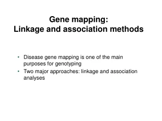
Linkage Vs. Association • Linkage: -Disease travels with marker within families -No association within individuals -Signals for complex traits are wide (20MB) • Association: -Can use case/control or case/parents design -Only works if association in the population -Allelic heterogeneity (eg, BRAC1) a problem • Linkage – large scale; Association fine scale (<200kb)
LOD Score • LOD score is log10 (odds for linkage/odds for no linkage) Traditional (1955) cut-off is LOD=3 (linkage 1000 times more likely) • A LOD of 3 corresponds to α = 0.0001 • Lander and Kruglyak (1995) A LOD score cut-off of 3.6 for a genome screen using an infinitely dense map corresponds to a “genome-wide significance of 0.05” • This is the criteria often cited today
Bipolar Disorder • Lifetime prevalence of BP1 ≈ 1%, BPII ≈ 0.5% • Risk of suicide 10 – 15% • Treatment not curative, treatments not completely effective in mitigating symptoms • Heritability estimates ≈ 80% • Linkage reports for ½ the chromosomes, with a lack of replication • Lack of power in original reports?
Significant and Suggestive Linkage • Given density of markers, significant linkage is LOD > 3.03 • Suggestive linkage is LOD > 1.75 • These take into account that 2 genome screens were analyzed (narrow and broad) • Significant – Occurs once in twenty genome screens Suggestive – Occurs once in a genome screen
Linkage Analysis (Summary) • Approximately 2,000 “independent “ tests with an infinitely dense genetic map (Multiple testing a much bigger problem in GWAS) • Linkage studies have been unsuccessful for complex diseases • May be useful as input into GWAS analysis? • Today – GWAS (using SNP chips) have taken over • My opinion – pursue chromosomes 6 and 8, even if not genome-wide significant in GWAS
Genome-Wide Association Studies (GWAS) • Chips by Illumina and Affymetrix genotype 1 million SNPs (Single Nucleotide Polymorphisms) as well as CNVs (Copy Number Variations) • Affordable on a large scale • Capitalize on Linkage Disequilibrium between the markers and variation at a susceptibility gene
Disequilibrium Let P(A1)=p1 Let P(B1)=q1 Let P(A1B 1)=h11 No association if h11=p1q1 D = h11-p1q1
Population Stratification Population 1 Population 2 Odds ratio = 1 Odds ratio = 1 Combined Population Odds ratio = 2.38
D´ and r² D tends to take on small values and depends on marginal gene frequencies D = D / max(D) r² = D² / (p1p2 q1q2) = square of usual correlation coefficient () Note: r2 = 0 D = 0 D = ±1 if one cell is zero (eg, no recombination) r² can be small even when D = ±1 Prediction of one SNP by another depends on r²
Haplotypes • We measure genotypes • A double heterozygote is ambiguous • Must estimate haplotype frequencies from genotype frequencies – usually assume random mating and use EM algorithm • The program haploview is commonly used to estimate and depict LD
Different Haplotypes; same genotypes A1 A2 B1 B2 • Haplotypes A1 B1, A2 B2; A1 B2, A2 B1 • Independence hij = pi qj • Positive Association hij > pi qj • Negative Association hij < pi qj
Blocks and Bins • Predictability of one SNP by another best described by r2 – basic statistics • Block – set of SNPs with all pair-wise LD high (usually defined in terms of D) • If one uses r2 – insert a SNP with low frequency in between SNPs with freqs close to 0.5, then block breaks up! • Perlegen (Hinds et al, Science, 2005) -– use bins where a tag SNP has r2 of 0.8 with all other SNPs. Bins may not be contiguous.
Summary (Blocks and Bins) • Blocks using D may have a “biological” interpretation (long stretches with |D | =1 and indicates no recombination) • Selection of Tag SNPs is a statistical issue, want to predict untyped SNPS from those that are typed – r2 is natural measure • Most current WGA studies use bins based on r2 (typically r2 > 0.8) • Sample size needed is N/ r2 with reduced r2
Analysis • Case/ control studies are common. Use logistic regression with case/control status as the dependent variable. Use SNP genotype as an independent variable with other covariates and test one SNP at a time • PLINK is my program of choice to do this • Family based studies are also used. TDT (case and both parents) designs are used in GWAS but less efficient
Testing Marker Effects log (odds) = + 1X1 odds = ee 1 X1 Genotype Odds 11 e 12 ee1 22 ee21 Test 1 = 0, all odds = e Note: No dominance effect
Testing Marker Effects log (odds) = + 1 X1 + 2 X2 odds = ee 1 X1 e 2 X2 Genotype Odds 1 1 e 1 2 e e1e2 2 2 ee21 Test 1= 2 = 0, all odds = e If 2 = 0, then have additive model
Haplotypes? • We may wish to consider more than one SNP at a time in the linear regression. • More information in a set of close SNPs • May wish to study a set of SNPs to see if one explains the case/control difference, i.e., does the evidence for one SNP disappear when controlling for other SNPs.
Haplotype Trend Analysis • Zaykin et al (2002) Hum Hered 53:79-91 • Use haplotypes in logistic regression • For a pair of SNPs, there are 4 haplotypes, so there will be 3 “dummy” variables • Assume pair of haplotypes in an individual are “additive”, so only need 3 regression coefficients • If haplotypes are known with certainty, then:
Estimated Haplotypes • One can get estimates of the haplotype probabilities for each individual (LD between SNPs OK) • Put the estimated probabilities into the logistic regression
GWAS Studies How do we keep up?
A Catalog of Published GWAS • www.genome.gov/26525384 • Number of Studies: • 2005 2 – Includes Age-related Macular Degeneration • 2006 8 • 2007 87 • 2008 70 (through July 27) • Bipolar Disorder: • 3 studies (1 used pooled genotypes) • No convincing signals
“History” of GWAS • Early studies used pooled designs – too expensive to do individual genotypes • Affymetrix and Illumina come out with affordable SNP chips • First study to generate enthusiasm – Age-related macular degeneration (Klein, 2007) found a “real” signal • Type II diabetes studies found “real” signals – linkage studies were problematic
Welcome Trust (WTCCC) Initiative • Common set of 3,000 controls • Several disorders (including Bipolar) with 2,000 cases each • Results in the public domain • Published in Nature in 2007
Major U.S. GWAS Initiatives • New NIH Policy – All NIH Funded GWAS studies must deposit individual genotypes and phenotypic data in dbGaP at NCBI • GAIN and GEI RFAs funded studies with existing DNA, subjects consented to allow data to go to dbGaP, and genotyping done at associated genotyping centers • New RFA from NIMH to collect very large (~10,000) samples
GAIN ProposalsGenetic Association Information Network • 6 WGA projects were selected across NIH • Projects: • Schizophrenia • Bipolar Disorder • Depression • ADHD • Psoriasis • Type 1 Diabetes (nephropathy) • Data at dbGap (1 year embargo on publication) • Note: 4/6 Mental Health related!!
Gene Environment Initiative (GEI) • 8 GWAS funded – oral cleft, addiction, coronary heart disease, lung cancer, type 2 diabetes, birth weight, dental caries, premature birth • Required existing DNA and subjects consented to share • Issued Supplement for replication samples • Addiction (Bierut) samples genotyped first – we got genotypes from CIDR in May; once cleaned, they go to dbGaP
Good News for Analysts • Cleaned data available goes to investigators who collected data at the same time as everyone else • It takes years to collect subjects • Cleaning GWAS data is hard and time consuming • Opportunity for combining data from multiple studies • Is this fair?
dbGaP • Genotype and Phenotype Database • Data made available to investigators and others at the same time – 1 year publication embargo • Request access using eRA Commons sign on – requires Institutional sign-off • Request must be approved by a DAC (data access committee)