Electrical Network Analysis Techniques and Theorems
Explore resistive network analysis including nodal and mesh analysis, Kirchhoff's laws, Thévenin and Norton theorems, maximum power transfer, and nonlinear elements in a linear circuit. Learn to solve complex circuits graphically and analytically.

Electrical Network Analysis Techniques and Theorems
E N D
Presentation Transcript
CHAPTER3 Resistive Network Analysis
Figure 3.2 Branch current formulation in nodal analysis Figure 3.2 3-1
Figure 3.3 Use of KCL in nodal analysis 3-2
Figure 3.4 Illustration of nodal analysis Figure 3.4 3-3
Figure 3.6 Figure 3.6 3-4
Figure 3.11 Circuit for Example 3.6 Figure 3.11 3-5
Figure 3.12 Basic principle of mesh analysis Figure 3.12 3-6
Figure 3.13 Use of KVL in mesh analysis Figure 3.13 3-7
Figure 3.14 A two-mesh circuit 3-8
Figure 3.15 Assignment of currents and voltages around mesh 1 Figure 3.15 3-9
Figure 3.17, 3.18 Figure 3.17 Figure 3.18 3-10
Figure 3.21 Circuit used to demonstrate mesh analysis with current sources Figure 3.21 3-11
Figure 3.25 Figure 3.25 3-12
Figure 3.27 The principle of superposition Figure 3.27 3-13
Figure 3.28 Zeroing voltage and current sources Figure 3.28 3-14
Figure 3.34, 3.35 Illustration of Thévenin theorem Figure 3.34 Illustration of Norton theorem Figure 3.35 3-15
Figure 3.36, 3.37 Computation of Thévenin resistance Equivalent resistance seen by the load Figure 3.36 Figure 3.37 3-16
Figure 3.43 Equivalence of open-circuit and Thévenin voltage Figure 3.43 3-17
Figure 3.47 A circuit and its Thévenin equivalent Figure 3.47 3-18
Figure 3.54 Computation of Norton current Figure 3.54 3-19
Figure 3.67 Measurement of open-circuit voltage and short-circuit current Figure 3.67 3-20
Power transfer between source and load Graphical representation of maximum power transfer Figure 3.69 Figure 3.70 3-21
Figure 3.73, 3.74 The i-v characteristic of exponential resistor Representation of nonlinear element in a linear circuit Figure 3.73 Figure 3.74 3-22
Figure 3.75, 3.76 Load line Figure 3.75 Graphical solution of equations 3.44 and 3.45 Figure 3.76 3-23