Key Concepts in Network Analysis: Understanding Structure and Dynamics
This document covers essential concepts in network analysis, focusing on key measures such as degree, degree distribution, average path length, shortest path length, clustering coefficient, modularity, and centrality measures. It elaborates on the characteristics of directed and undirected networks, explores network models including random and scale-free networks, and discusses the generation of graphs using the Erdős-Rényi and Barabási-Albert models. The discussion highlights the significance of clustering coefficients and path lengths in analyzing network properties and dynamics.

Key Concepts in Network Analysis: Understanding Structure and Dynamics
E N D
Presentation Transcript
Network analysis Sushmita Roy BMI/CS 576 www.biostat.wisc.edu/bmi576 sroy@biostat.wisc.edu Dec 3rd, 2013
Key concepts • Network measures • Degree • Degree distribution • Average path length and shortest path length • Clustering coefficient • Modularity • Network motifs • Centrality measures • Network models • Random networks • Scale free networks
Directed and undirected networks Vertex/Node A A E E D F D F Edge Directed Edge B B C C Undirected network Directed network
Node degree • Undirected network • Degree, k: Number of neighbors of a node • Directed network • Indegree, kin: Number of incoming edges • Out degree, kout: Number of outgoing edges • Average degree (undirected network) A E Indegree of F is 4 Outdegree of E is 1 D F Directed Edge B C
Average degree • Consider an undirected network with N nodes and L edges • Let ki denote the degree of node i • Average degree is • Average degree is equivalently defined as
Degree distribution • P(k) gives the probability that a selected node has k edges • Different networks can have different degree distributions • A fundamental property that can be used to characterize a network
Different degree distributions • Poisson distribution • The mean is a good representation of ki of all nodes • Exhibited in ErdosRenyi networks • Power law distribution • Also called scale free • There is no “typical” node that captures the degree of nodes.
Poisson distribution • A discrete distribution • The Poisson is parameterized by which can be easily estimated by maximum likelihood P(X=k) k
Power law distribution • Used to capture the degree distribution of most biological/real networks • Typical value of is between 2 and 3. • MLE exists for but is more complicated • See Power-Law Distributions in Empirical Data. Clauset, Shalizi and Newman, 2009 for details P(k)
ErdosRenyi random graphs • Dates back to 1960 due to two mathematicians Paul Erdos and Alfred Renyi. • Provides a probabilistic model to generate a graph • Starts with N nodes and connects two nodes with probability p • Node degrees follow a Poisson distribution • Tail falls off exponentially, suggesting that nodes with degrees different from the mean are very rare
Generating a graph using the ER model • Input • p: probability of an edge • N: number of nodes in the network • Output: An ER network of N nodes with on p*N(N-1)/2 edges on average • For each possible edge add with probability p
Scale free networks • Degree distribution is captured by a power law distribution • Such networks are ubiquitous in nature • Scale-free networks can be generated by the preferential attachment model from Barabasi-Albert • A “rich gets richer” model
Generating a Scale free network with the preferential attachment model • Input: • N: number of nodes • m: number of existing nodes to connect • Output: a scale-free network • At each iteration • Add a node with m connections • Select a node i as one of the m neighbors with probability
Poisson versus Scale free Barabasi & Oltvai
Path lengths • The shortest path length between two nodes A and B: • The smallest number of edges that need to be traversed to get from A to B • Mean path length is the average of all shortest path lengths • Diameter of a graph is the longest of all shortest paths in the network
Scale-free networks are ultra-small • Average path length is log log N • In a random network (ErdosRenyi network) the average path length is log N
Clustering coefficient • Measure of transitivity in the network • If A is connect to B, and B is connected to C, how often is A connected to C • Clustering coefficient Ci for each node i is • niis the number of edges among neighbors of i • The ratio of the number of edges connecting i’s neighbors to the max possible • Average clustering coefficient gives a measure of nodes to form clusters B C A ?
Clustering coefficient example G B A C D
Let’s look at some large networks • We will consider networks of 800-1000 nodes • One is generated using the Preferential attachment model • One is generated using the ER model
Networks generated from the different models ER random network Preferential attachment
Degree distributions of the two networks Preferential attachment ER random network
Relationship between clustering coefficient and degree • Define C(k) as the average clustering coefficient of all nodes with degree k • In some networks • If this is true, the networks are said to have a hierarchical organization • Smaller node sets are linked together to form larger modules.
Hierarchical network A hierarchical network generated by replicating the current set of nodes Scale-free distribution of degrees Inverse relationship between C(k) and degree Barabasi & Oltvai, 2004
Hierarchical organization is seen also among nodes • Regulators are hierarchically organized with different roles per level • Top: Master regulators influence many genes • Middle: Bottle necks directly targeting most genes • Bottom: Essential regulators Hierarchical structure of S. cerevisiaeregulatory network Yu & Gerstein 2006, Jothi et al. 2009
Given a network how can we test what degree distribution it follows? • Compute the empirical degree distribution • Degree distribution can Poisson or Power law • Estimate parameters of the distribution from the data • Pick the distribution that fits the data better.
Properties of scale free networks • Degree distribution is best captured by a power law distribution • Average clustering coefficient is higher than expected from a random network • Average path length is smaller than expected from a random network
Centrality measures in networks • A measure of how important network node is • Four types of centrality measures defined for each node • Degree centrality • The degree of a node • Betweenness centrality • The number of shortest paths between two nodes that passes through the node of interest • Closeness centrality • Sum of a distances from other nodes • Eigenvector centrality • Given by the largest eigen vector of the adjacency matrix
Eigenvector centrality • Based on the idea that nodes with high score should influence the importance of a node more • Given by • The centrality measures are given by the entries of the first eigen vector • Google’s page rank algorithm makes use of a type of Eigen vector centrality Largest eigen value Neighbors of v
Degree centrality of a node is correlated to functional importance of a node Yeast protein-protein interaction network Red nodes on deletion cause the organism to die Red nodes also among the most degree central
Network motifs • Degree distributions capture important global properties of the network • Can we say something about more local properties of the network? • Network motifs are defined as small recurring subnetworks that occur much more than a randomized network • A subgraph is called a network motif of a network if its occurrence in randomized networks is significantly less than the original network. • Some motifs are associated to explain specific network dynamics Milo Science 2002
Finding network motifs • Enumerating motifs • Subgraph enumeration • Calculating the number of occurrences in randomized networks Milo 2002
Network motifs found in many complex networks The occurrence of the feedforward loop in both networks suggests a fundamental similarity in the design on these networks
Structural common motifs seen in the yeast regulatory network Auto-regulation Multi-component Feed-forward loop Single Input Multi Input Regulatory Chain Feed-forward loops involved in speeding up in response of target gene Lee et.al. 2002,Mangan & Alon, 2003
Modularity in networks • Modularity “refers to a group of physically or functionally linked nodes that work together to achieve a distinct function” -- Barabasi & Oltvai • Similar idea is captured by the “community structure” in networks • Two questions • Given a network is it modular? • Given a network what are the modules in the network?
A modular network Module 2 Module 3 Module 1
Assessing the modularity of a network • Modularity of a network can be assessed in two ways: • Recall the average clustering coefficient • A modular network is one that has a significantly higher clustering coefficient than a network with equivalent number of nodes and degree distribution • If we know an existing grouping of nodes, we can compute modularity (Q) as • difference between within group (community) connections and expected connections within a group Q defined as in: Finding and evaluating community structure in networks, http://arxiv.org/abs/cond-mat/0308217v1
Finding modules in a graph • Given a graph find the densely connected subgraphs • Graph clustering algorithms are applicable here • Hierarchical clustering using the edge weight as a distance • How to define weight? • Markov clustering algorithm • Girvan-Newman algorithm
Girvan-Newman algorithm • Initialize • Compute betweennees for all edges • Repeat until convergence criteria • Remove the node with the highest betweennees • Recomputebetweenness of affected edges • Convergence criteria can be • No more edges • Desired modularity.
Zachary’s karate club study Node grouping based on betweenness Each node is an individual and edges represent social interactions among individuals. The shape and colors represent different groups.
Summary of network analysis • Given a network, its topology can be characterized using different measures • Degree distribution • Average path length • Clustering coefficient • Centrality measures • Allow us to assess the importance of different nodes • Network motifs • Overrepresentation of subgraphs of specific types • Network modularity