Download
1 / 7
70 likes | 176 Vues
This document showcases a comparison of various plots generated from both traditional and modern Roman Pot configurations used in high-energy physics experiments. It provides detailed equations for each Roman Pot setup, illustrating how combining two pots leads to a system of four equations with four unknowns. The analysis includes mean displacement values across different configurations and discusses data distribution, aligning with historical context from a presentation on October 21, 2009. The insights help understand particle scattering processes effectively.

E N D
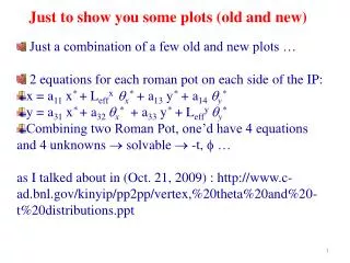
Just to show you some plots (old and new) • Just a combination of a few old and new plots … • 2 equations for each roman pot on each side of the IP: • x = a11 x*+ Leffxx* + a13 y* + a14y* • y = a31 x*+ a32 x* + a33 y* + Leffy y* • Combining two Roman Pot, one’d have 4 equations and 4 unknowns solvable -t, … • as I talked about in (Oct. 21, 2009) : http://www.c-ad.bnl.gov/kinyip/pp2pp/vertex,%20theta%20and%20-t%20distributions.ppt
The “mean” is now in the order of magnitude of 0.x mm. • x(EVU-WVD) ~1.6 mm • y(EVU-WVD) ~0.2 mm • x(EVD-WVU) ~0.3 mm • y(EVD-WVU) ~0.3 mm • Before alignment, it’s ~ some mm.
-t = 4P02Sin2(/2) , P0 = 100. 21557 calculated from B and G =191.500006443 in RampEditor (of C-AD) -t distribution without any collinearity cut After loose collinearity cut
=Tan-1(Py/Px) without collinearity cut with loose collinearity cut
Frac. of golden events / triggered events : • Runs with loose collinearity cut • 10182025 71% 65% • 10183035 78% 74% • 10183037 77% 73%