Chapter 8. FIR Filter Design
Chapter 8. FIR Filter Design. Gao Xinbo School of E.E., Xidian Univ. xbgao@ieee.org http://see.xidian.edu.cn/teach/matlabdsp/. Introduction. In digital signal processing, there are two important types of systems: Digital filters : perform signal filtering in the time domain


Chapter 8. FIR Filter Design
E N D
Presentation Transcript
Chapter 8. FIR Filter Design Gao Xinbo School of E.E., Xidian Univ. xbgao@ieee.org http://see.xidian.edu.cn/teach/matlabdsp/
Introduction • In digital signal processing, there are two important types of systems: • Digital filters: perform signal filtering in the time domain • Spectrum analyzers: provide signal representation in the frequency domain • In this and next chapter we will study several basic design algorithms for both FIR and IIR filters. • These designs are mostly of the frequency selective type • Multiband lowpass, highpass, bandpass and bandstop filters
Introduction • In FIR filter design we will also consider systems like differentiators or Hilbert transformers. • It is not frequency selective filters • Nevertheless follow the design techniques being considered. • We first begin with some preliminary issues related to design philosophy and design specifications. These issues are applicable to both FIR and IIR filter designs. • We will study FIR filter design algorithms in the rest of this chapter.
Preliminaries • The design of a digital filter is carried out in three steps: • Specifications: they are determined by the applications • Approximations: once the specification are defined, we use various concepts and mathematics that we studied so far to come up with a filter description that approximates the given set of specifications. (in detail) • Implementation: The product of the above step is a filter description in the form of either a difference equation, or a system function H(z), or an impulse response h(n). From this description we implement the filter in hardware or through software on a computer.
Specifications • Specifications are required in the frequency-domain in terms of the desired magnitude and phase response of the filter. Generally a linear phase response in the passband is desirable. • In the case of FIR filters, It is possible to have exact linear phase. • In the case of IIR filters, a linear phase in the passband is not achievable. • Hence we will consider magnitude-only specifications.
Magnitude Specifications • Absolute specifications • Provide a set of requirements on the magnitude response function |H(ejw)|. • Generally used for FIR filters. • Relative specifications • Provide requirements in decibels (dB), given by • Used for both FIR and IIR filters.
Absolute specifications of a lowpass filter Passband ripple Transition band Stopband ripple
Absolute Specifications • Band [0,wp] is called the passband, and delta1 is the tolerance (or ripple) that we are willing to accept in the ideal passband response. • Band [ws,pi] is called the stopband, and delta2is the corresponding tolerance (or ripple) • Band [wp, ws] is called the transition band, and there are no restriction on the magnitude response in this band.
0 Relative (DB) Specifications
Relations between specifications • Ex7.1 & ex7.2 calculation of Rp and As
Why we concentrate on a lowpass filter? • The above specifications were given fro a lowpass filter. • Similar specifications can also be given for other types of frequency-selective filters such as highpass or bandpass. • However, the most important design parameters are frequency-band tolerance (or ripples) and band-edge frequencies. • Whether the given band is a passband or stopband is a relatively minor issue.
Problem statement • Design a lowpass filter (i.e., obtain its system function H(z) or its difference equation) that has a passband [0,wp] with tolerance delta1 (or Rp in dB) and a stopband [ws,pi] with tolerance delta2 (or As in dB)
Design and implementational advantages of the FIR digital filter • The phase response can be exactly linear; • They are relatively easy to design since there are no stability problems. • They are efficient to implement; • The DFT can be used in their implementation.
Advantages of a linear-phase response • Design problem contains only real arithmetic and not complex arithmetic; • Linear-phase filter provide no delay distortion and only a fixed amount of delay; • For the filter of length M (or order M-1) the number of operations are of the order of M/2 as we discussed in the linear phase implementation.
Properties of Linear-phase FIR Filter • Let h(n), n=0,1,…,M-1 be the impulse response of length (or duration) M. Then the system function is Which has (M-1) poles at the origin (trivial poles) and M-1 zeros located anywhere in the z-plane. The frequency response function is
Impulse Response h(n) • We impose a linear-phase constraint Where alpha is a constant phase delay. Then we know from Ch6 that h(n) must be symmetric, that is Hence h(n) is symmetric about alpha, which is the index of symmetry. There are two possible types of symmetry:
A second type of linear-phase FIR filter • The phase response satisfy the condition Which is a straight line but not through the origin. In this case alpha is not a constant phase delay, but Is constant, which is the group delay. Therefore alpha is a constant group delay. In this case, as a group, frequencies are delayed at a constant rate.
A second type of linear-phase FIR filter • For this type of linear phase one can show that This means that the impulse response h(n) is antisymmetric. The index of symmetry is still alpha=(M-1)/2. Once again we have two possible types, one for M odd and one for M even. Figure P230
Frequency Response H(ejw) • When the case of symmetry and anti-symmetry are combined with odd and even M, we obtain four types of linear phase FIR filters. Frequency response functions for each of these types have some peculiar expressions and shapes. To study these response, we write H(ejw) as Hr(ejw) is an amplitude response function and not a magnitude response function. The phase response associated with the magnitude response is a discontinuous function, while that associated with the amplitude response is a continuous linear function.
Type-1 Linear-phase FIR filter: Symmetrical impulse response, M odd In this case, beta=0, alpha=(M-1)/2 is an integer, and h(n)=h(M-1-n), 0<=n<=M-1. Then
Type-2 Linear-phase FIR filter: Symmetrical impulse response, M even In this case, beta=0, h(n)=h(M-1-n), 0<=n<=M-1, but alpha=(M-1)/2 is not an integer, and then Note that Hr(pi)=0, hence we cannot use this type for highpass or bandstop filters.
Type-3 Linear-phase FIR filter: Antisymmetric impulse response, M odd In this case, beta=pi/2, alpha=(M-1)/2 is an integer, and h(n)=-h(M-1-n), 0<=n<=M-1. Then Hr(0)=Hr(pi)=0, hence this type of filter is not suitable for designing a lowpass filter or a highpass filter.
Type-4 Linear-phase FIR filter: Antisymmetric impulse response, M even This case is similar to Type-2. We have Hr(0)=0 and exp(jpi/2)=j. Hence this type of filter is also suitable for designing digital Hilbert transforms and differentiators.
Matlab Implementation • Hr-type 1 • Hr-type 2 • Hr-type 3 • Hr-type 4
Zeros quadruplet for linear-phase filters • For real sequence, zeros are in conjudgates; • For symmetry sequence, zeros are in mirror; • Substitute q=z –1, the polynomial coefficients for q are in reverse order of polynomial of z. • Since coefficients h(n) are symmetry, reverse in order do not change the coefficients vector. • If zk is a root of the polynomial, thus pk=zk-1 is also a root.
Mirror zeros for symmetry coef.. • If zk satisfy polynomial: h0+h1zk-1+ h2zk-2 +..+ hM-2zk-M+2 + hM-1zk-M+1=0 where hM-1=h0 ,hM-2 =h1,… Then rk = zk–1 satisfy the same equation h0+h1rk+ h2rk2 + …+ h1rkM-2 + h0rkM-1 = h0zkM-1 + h1zkM-2 + … + h2zk2+ h1zk + h0 = = zkM-1(h0+ h1zk-1 + …+ h1zk-M+2 + h0zk –M+1) =0
1/Conj(Z1) Z1 Conj(Z1) 1/z1
Examples • Examples7.4 • Examples7.5 • Examples7.6 • Examples7.7
Windows Design Techniques • Basic idea: choose a proper ideal frequency-selective filter (which always has a noncausal, infinite-duration impulse response) and then truncate (or window) its impulse response to obtain a linear-phase and causal FIR filter. • Appropriate windowing function • Appropriate ideal filter • An ideal LPF of bandwidth wc<pi is given by Where wc is also called the cutoff frequency, alpha is called the sample delay
Windows Design Techniques Note that hd(n) is symmetric with respect to alpha, a fact useful for linear-phase FIR filter. To obtain a causal and linear-phase FIR filter h(n) of length M, we must have This operation is called “windowing”.
Windowing Depending on how we define w(n) above, we obtain different window design. For example, W(n) = RM(n), rectangular window This is shown pictorially in Fig.7.8.
Observations: • Since the window w(n) has a finite length equal to M, its response has a peaky main lobe whose width is proportional to 1/M, and its side lobes of smaller heights. • The periodic convolution produces a smeared version of the ideal response Hd(ejw) • The main lobe produces a transition band in H(ejw) whose width is responsible for the transition width. This width is then proportional to 1/M. the wider the main lobe, the wider will be the transition width. • The side lobes produce ripples that have similar shapes in both the passband and stopband.
Basic Window Design Idea • For the given filter specifications choose the filter length M and a window function w(n) for the narrowest main lobe width and the smallest side lobe attenuation possible. • From the observation 4 above we note that the passband tolerance delta1 and the stopband tolerance delta2 can not be specified independently. We generally take care of delta2 alone, which results in delta2 = delta1.
Rectangular Window This is the simplest window function but provides the worst performance from the viewpoint of stopband attenuation. Figure 7.9
Observations: • The amplitude response Wr(w) has the first zero at w=w1=2pi/M. Hence the width of the main lobe is 2w1=4pi/M. Therefore the approximate transition bandwidth is 4pi/M. • The magnitude of the first side lobe (the peak side lobe magnitude) is approximately at w=3pi/M and is given by |Wr(3pi/M)| = 2M/(3pi), for M>>1. Comparing this with the main lobe amplitude, which is equal to M, the peak side lobe magnitude is 2/(3pi)=21.11%=13dB of the main lobe amplitude.
Observations • The accumulated amplitude response has the first side lobe magnitude at 21dB. This results in the minimum stopband attenuation of 21dB irrespective of the window length M. • Using the minimum stopband attenuation, the transition bandwidth can be accurately computed. This computed exact transition bandwidth is ws-wp = 1.8pi/M, which is about half the approximate bandwidth of 4pi/M.
Two main problems • The minimum stopband attenuation of 21dB is insufficient in practical applications. • The rectangular windowing being a direct truncation of the infinite length hd(n), it suffers from the Gibbs phenomenon.
Bartlett Window • Bartlett suggested a more gradual transition in the form of a triangular window Figure 7.11
Hanning Window • This is a raised cosine window function. Hamming Window:
Blackman Window Kaiser Window: I0[] is the modified zero-order Bessel function
Kaiser Window If beta=5.658, then the transition width is equal to 7.8pi/M, and the minimum stopband attenuation is equal to 60dB. If beta=4.538, then the transition width is equal to 5.8pi/M, and the minimum stopband attenuation is equal to 50dB. KAISER HAS DEVELOPED EMPIRICAL DESIGN EQUATIONS.
滤波器阶数(长度)M的选择 取Kaiser窗时设定beta,再用kaiserord函数求得M
Matlab Implementation • W=boxcar(M): rectangular window • W=triang(M): bartlett window • W=hanning(M) • W=hamming(M) • W=blackman(M) • W=kaiser(M,beta) • Examples
Frequency Sampling Design Techniques • In this design approach we use the fact that the system function H(z) can be obtained from the samples H(k) of the frequency response H(ejw). • This design technique fits nicely with the frequency sampling structure that we discussed in Ch6.
Phase for Type 1 & 2 Phase for Type 3 & 4
Frequency Sampling Design Techniques • Basic Idea: • Given the ideal lowpass filter Hd(ejw), choose the filter length M and then sample Hd(ejw) at M equispaced frequencies between 0 and 2pi. The actual response is the interpolation of the samples is given by
From Fig.7.25, we observe the following • The approximation error—that is difference between the ideal and the actual response—is zero at the sampled frequencies. • The approximation error at all other frequencies depends on the shape of the ideal response; that is, the sharper the ideal response, the larger the approximation error. • The error is larger near the band edge and smaller within the band.