Download
1 / 59
600 likes | 826 Vues
Lecture 25 Built-In Self-Testing Pattern Generation and Response Compaction. Motivation and economics Definitions Built-in self-testing (BIST) process BIST pattern generation (PG) BIST response compaction (RC) Aliasing probability Example Summary. BIST Motivation.

E N D
Lecture 25Built-In Self-TestingPattern Generation and Response Compaction • Motivation and economics • Definitions • Built-in self-testing (BIST) process • BIST pattern generation (PG) • BIST response compaction (RC) • Aliasing probability • Example • Summary VLSI Test: Bushnell-Agrawal/Lecture 25
BIST Motivation • Useful for field test and diagnosis (less expensive than a local automatic test equipment) • Software tests for field test and diagnosis: • Low hardware fault coverage • Low diagnostic resolution • Slow to operate • Hardware BIST benefits: • Lower system test effort • Improved system maintenance and repair • Improved component repair • Better diagnosis VLSI Test: Bushnell-Agrawal/Lecture 25
Costly Test Problems Alleviated by BIST • Increasing chip logic-to-pin ratio – harder observability • Increasingly dense devices and faster clocks • Increasing test generation and application times • Increasing size of test vectors stored in ATE • Expensive ATE needed for 1 GHz clocking chips • Hard testability insertion – designers unfamiliar with gate-level logic, since they design at behavioral level • In-circuit testing no longer technically feasible • Shortage of test engineers • Circuit testing cannot be easily partitioned VLSI Test: Bushnell-Agrawal/Lecture 25
Typical Quality Requirements • 98% single stuck-at fault coverage • 100% interconnect fault coverage • Reject ratio – 1 in 100,000 VLSI Test: Bushnell-Agrawal/Lecture 25
Design and test + / - + / - + / - Diagnosis and repair - - Fabri- cation + + + Manuf. Test - - - Maintenance test - Service interruption - Level Chips Boards System Benefits and Costs of BIST with DFT + Cost increase - Cost saving +/- Cost increase may balance cost reduction VLSI Test: Bushnell-Agrawal/Lecture 25
Economics – BIST Costs • Chip area overhead for: • Test controller • Hardware pattern generator • Hardware response compacter • Testing of BIST hardware • Pin overhead -- At least 1 pin needed to activate BIST operation • Performance overhead – extra path delays due to BIST • Yield loss – due to increased chip area or more chips In system because of BIST • Reliability reduction – due to increased area • Increased BIST hardware complexity – happens when BIST hardware is made testable VLSI Test: Bushnell-Agrawal/Lecture 25
BIST Benefits • Faults tested: • Single combinational / sequential stuck-at faults • Delay faults • Single stuck-at faults in BIST hardware • BIST benefits • Reduced testing and maintenance cost • Lower test generation cost • Reduced storage / maintenance of test patterns • Simpler and less expensive ATE • Can test many units in parallel • Shorter test application times • Can test at functional system speed VLSI Test: Bushnell-Agrawal/Lecture 25
Definitions • BILBO – Built-in logic block observer, extra hardware added to flip-flops so they can be reconfigured as an LFSR pattern generator or response compacter, a scan chain, or as flip-flops • Concurrent testing – Testing process that detects faults during normal system operation • CUT – Circuit-under-test • Exhaustive testing – Apply all possible 2npatterns to a circuit with n inputs • Irreducible polynomial – Boolean polynomial that cannot be factored • LFSR – Linear feedback shift register, hardware that generates pseudo-random pattern sequence VLSI Test: Bushnell-Agrawal/Lecture 25
More Definitions • Primitive polynomial – Boolean polynomialp (x)that can be used to compute increasing powersnofxn modulo p (x)to obtain all possible non-zero polynomials of degree less thanp (x) • Pseudo-exhaustive testing – Break circuit into small, overlapping blocks and test each exhaustively • Pseudo-random testing – Algorithmic pattern generator that produces a subset of all possible tests with most of the properties of randomly-generated patterns • Signature – Any statistical circuit property distinguishing between bad and good circuits • TPG – Hardware test pattern generator VLSI Test: Bushnell-Agrawal/Lecture 25
BIST Process • Test controller – Hardware that activates self-test simultaneously on all PCBs • Each board controller activates parallel chip BIST Diagnosis effective only if very high fault coverage VLSI Test: Bushnell-Agrawal/Lecture 25
BIST Architecture • Note: BIST cannot test wires and transistors: • From PI pins to Input MUX • From POs to output pins VLSI Test: Bushnell-Agrawal/Lecture 25
BILBO – Works as Both a PG and a RC • Built-in Logic Block Observer (BILBO) -- 4 modes: • Flip-flop • LFSR pattern generator • LFSR response compacter • Scan chain for flip-flops VLSI Test: Bushnell-Agrawal/Lecture 25
Complex BIST Architecture • Testing epoch I: • LFSR1 generates tests for CUT1 and CUT2 • BILBO2 (LFSR3) compacts CUT1 (CUT2) • Testing epoch II: • BILBO2 generates test patterns for CUT3 • LFSR3 compacts CUT3 response VLSI Test: Bushnell-Agrawal/Lecture 25
Bus-Based BIST Architecture • Self-test control broadcasts patterns to each CUT over bus – parallel pattern generation • Awaits bus transactions showing CUT’s responses to the patterns: serialized compaction VLSI Test: Bushnell-Agrawal/Lecture 25
Pattern Generation • Store in ROM – too expensive • Exhaustive • Pseudo-exhaustive • Pseudo-random (LFSR) – Preferred method • Binary counters – use more hardware than LFSR • Modified counters • Test pattern augmentation • LFSR combined with a few patterns in ROM • Hardwarediffracter – generates pattern cluster in neighborhood of pattern stored in ROM VLSI Test: Bushnell-Agrawal/Lecture 25
Exhaustive Pattern Generation • Shows that every state and transition works • For n-input circuits, requires all 2n vectors • Impractical for n > 20 VLSI Test: Bushnell-Agrawal/Lecture 25
Pseudo-Exhaustive Method • Partition large circuit into fanin cones • Backtrace from each PO to PIs influencing it • Test fanin cones in parallel • Reduced # of tests from 28 = 256 to 25 x 2 = 64 • Incomplete fault coverage VLSI Test: Bushnell-Agrawal/Lecture 25
Pseudo-Exhaustive Pattern Generation VLSI Test: Bushnell-Agrawal/Lecture 25
Random Pattern Testing Bottom: Random- Pattern Resistant circuit VLSI Test: Bushnell-Agrawal/Lecture 25
Pseudo-Random Pattern Generation • StandardLinear Feedback Shift Register (LFSR) • Produces patterns algorithmically – repeatable • Has most of desirable random # properties • Need not cover all 2n input combinations • Long sequences needed for good fault coverage VLSI Test: Bushnell-Agrawal/Lecture 25
Matrix Equation for Standard LFSR 0 0 . . . 0 0 1 X0 (t + 1) X1 (t + 1) . . . Xn-3 (t + 1) Xn-2 (t + 1) Xn-1 (t + 1) 0 1 . . . 0 0 h2 … … … … … 0 0 . . . 1 0 hn-2 0 0 . . . 0 1 hn-1 X0 (t) X1 (t) . . . Xn-3 (t) Xn-2 (t) Xn-1 (t) 1 0 . . . 0 0 h1 = X (t + 1) = Ts X (t) (Ts is companion matrix) VLSI Test: Bushnell-Agrawal/Lecture 25
LFSR Implements a Galois Field • Galois field (mathematical system): • Multiplication by x same as right shift of LFSR • Addition operator is XOR () • Ts companion matrix: • 1st column 0, except nth element which is always 1 (X0 always feeds Xn-1) • Rest of row n – feedback coefficients hi • Rest is identity matrix I – means a right shift • Near-exhaustive (maximal length) LFSR • Cycles through 2n – 1 states (excluding all-0) • 1 pattern of n 1’s, one of n-1 consecutive 0’s VLSI Test: Bushnell-Agrawal/Lecture 25
Standard n-Stage LFSR Implementation • Autocorrelation – any shifted sequence same as original in 2n-1 – 1 bits, differs in 2n-1 bits • If hi = 0, that XOR gate is deleted VLSI Test: Bushnell-Agrawal/Lecture 25
LFSR Theory • Cannot initialize to all 0’s – hangs • If X is initial state, progresses through states X, Ts X, Ts2 X, Ts3 X, … • Matrix period: Smallest k such that Tsk = I • k LFSR cycle length • Described by characteristic polynomial: f (x) = |Ts – I X | = 1 + h1x + h2x2 + … + hn-1xn-1 + xn VLSI Test: Bushnell-Agrawal/Lecture 25
LFSR Fault Coverage Projection • Fault detection probability by a random number p (x) dx = fraction of detectable faults with detection probability between x and x + dx • p (x) dx0 when 0 x 1 • p (x) dx = 1 • Exist p (x) dx faults with detection probability x • Mean coverage of those faults is x p (x) dx • Mean fault coverage yn of 1stn vectors: I (n) = 1 - (1 – x)np (x) dx yn 1 – I (n) + (15.6) 1 0 1 0 n total faults VLSI Test: Bushnell-Agrawal/Lecture 25
LFSR Fault Coverage & Vector Length Estimation • Random-fault-detection (RFD) variable: • Vector # at which fault first detected • wi # faults with RFD variablei • So p (x) =Swi pi (x) • ns size of sample simulated; N # test vectors • w0 ns-S wi • Method: • Estimate random first detect variables wi from fault simulator using fault sampling • Estimate I (n) using book Equation 15.8 • Obtain test length by inverting Equation 15.6 & solving numerically N 1 ns i = 1 N i = 1 VLSI Test: Bushnell-Agrawal/Lecture 25
Example External XOR LFSR • Characteristic polynomial f (x) = 1 + x + x3 (read taps from right to left) VLSI Test: Bushnell-Agrawal/Lecture 25
X0 X1 X2 1 0 0 0 0 1 0 1 0 1 0 1 0 1 1 1 1 1 1 1 0 1 0 0 0 0 1 X0 (t + 1) X1 (t + 1) X2 (t + 1) 0 0 1 1 0 1 0 1 0 X0 (t) X1 (t) X2 (t) = External XOR LFSR • Pattern sequence for example LFSR (earlier): • Always have 1 and xn terms in polynomial • Never repeat an LFSR pattern more than 1 time –Repeats same error vector, cancels fault effect … VLSI Test: Bushnell-Agrawal/Lecture 25
Generic Modular LFSR VLSI Test: Bushnell-Agrawal/Lecture 25
Modular Internal XOR LFSR • Described by companion matrixTm = TsT • Internal XOR LFSR – XOR gates in between D flip-flops • Equivalent to standard External XOR LFSR • With a different state assignment • Faster – usually does not matter • Same amount of hardware • X (t + 1) = Tm x X (t) • f (x) = | Tm – I X | = 1 + h1 x + h2x2 + … + hn-1xn-1 + xn • Right shift – equivalent to multiplying by x, and then dividing by characteristic polynomial and storing the remainder VLSI Test: Bushnell-Agrawal/Lecture 25
Modular LFSR Matrix 0 1 0 . . . 0 0 0 X0 (t + 1) X1 (t + 1) X2 (t + 1) . . . Xn-3 (t + 1) Xn-2 (t + 1) Xn-1 (t + 1) 0 0 1 . . . 0 0 0 0 0 0 . . . 0 0 0 … … … … … … 0 0 0 . . . 0 1 0 0 0 0 . . . 0 0 1 X0 (t) X1 (t) X2 (t) . . . Xn-3 (t) Xn-2 (t) Xn-1 (t) 1 h1 h2 . . . hn-3 hn-2 hn-1 = VLSI Test: Bushnell-Agrawal/Lecture 25
Example Modular LFSR • f (x) = 1 + x2 + x7 + x8 • Read LFSR tap coefficients from left to right VLSI Test: Bushnell-Agrawal/Lecture 25
Primitive Polynomials • Want LFSR to generate all possible 2n – 1 patterns (except the all-0 pattern) • Conditions for this – must have a primitive polynomial: • Monic – coefficient of xn term must be 1 • Modular LFSR – all D FF’s must right shift through XOR’s from X0 through X1, …, through Xn-1, which must feed back directly to X0 • Standard LFSR – all D FF’s must right shift directly from Xn-1 through Xn-2, …, through X0, which must feed back into Xn-1 through XORing feedback network VLSI Test: Bushnell-Agrawal/Lecture 25
Primitive Polynomials (continued) • Characteristic polynomial must divide the polynomial 1 + xk for k = 2n – 1, but not for any smaller k value • See Appendix B of book for tables of primitive polynomials • If p (error) = 0.5, no difference between behavior of primitive & non-primitive polynomial • But p (error) is rarely = 0.5 In that case, non-primitive polynomial LFSR takes much longer to stabilize with random properties than primitive polynomial LFSR VLSI Test: Bushnell-Agrawal/Lecture 25
s-a-0 F Weighted Pseudo-Random Pattern Generation • If p (1) at all PIs is 0.5, pF (1) = 0.58 = • Will need enormous # of random patterns to test a stuck-at 0 fault on F -- LFSR p (1) = 0.5 • We must not use an ordinary LFSR to test this • IBM – holds patents on weighted pseudo-random pattern generator in ATE 1 256 f 1 256 255 256 pF (0) = 1 – = VLSI Test: Bushnell-Agrawal/Lecture 25
Weighted Pseudo-Random Pattern Generator • LFSR p (1) = 0.5 • Solution: Add programmable weight selection and complement LFSR bits to get p (1)’s other than 0.5 • Need 2-3 weight sets for a typical circuit • Weighted pattern generator drastically shortens pattern length for pseudo-random patterns VLSI Test: Bushnell-Agrawal/Lecture 25
w1 0 0 0 0 w2 0 0 1 1 Inv. 0 1 0 1 p (output) ½ ½ ¼ 3/4 w1 1 1 1 1 w2 0 0 1 1 Inv. 0 1 0 1 p (output) 1/8 7/8 1/16 15/16 Weighted Pattern Gen. VLSI Test: Bushnell-Agrawal/Lecture 25
Cellular Automata (CA) • Superior to LFSR – even “more” random • No shift-induced bit value correlation • Can make LFSR more random with linear phase shifter • Regular connections – each cell only connects to local neighbors xc-1 (t) xc (t) xc+1 (t) Gives CA cell connections 111 110 101 100 011 010 001 000 • xc (t + 1) 0 1 0 1 1 0 1 0 26 + 24 + 23 + 21 = 90 Called Rule 90 • xc (t + 1) = xc-1 (t) xc+1 (t) VLSI Test: Bushnell-Agrawal/Lecture 25
Cellular Automaton • Five-stage hybrid cellular automaton • Rule 150: xc (t + 1) = xc-1 (t) xc (t) xc+1 (t) • Alternate Rule 90 and Rule 150 CA VLSI Test: Bushnell-Agrawal/Lecture 25
Test Pattern Augmentation • Secondary ROM – to get LFSR to 100% SAF coverage • Add a small ROM with missing test patterns • Add extra circuit mode to Input MUX – shift to ROM patterns after LFSR done • Important to compact extra test patterns • Use diffracter: • Generates cluster of patterns in neighborhood of stored ROM pattern • Transform LFSR patterns into new vector set • Put LFSR and transformation hardware in full-scan chain VLSI Test: Bushnell-Agrawal/Lecture 25
Response Compaction • Severe amounts of data in CUT response to LFSR patterns – example: • Generate 5 million random patterns • CUT has 200 outputs • Leads to: 5 million x 200 = 1 billion bits response • Uneconomical to store and check all of these responses on chip • Responses must be compacted VLSI Test: Bushnell-Agrawal/Lecture 25
Definitions • Aliasing – Due to information loss, signatures of good and some bad machines match • Compaction – Drastically reduce # bits in original circuit response – lose information • Compression – Reduce # bits in original circuit response – no information loss – fully invertible (can get back original response) • Signature analysis – Compact good machine response into good machine signature. Actual signature generated during testing, and compared with good machine signature • Transition Count Response Compaction – Count # transitions from 0 1 and 1 0 as a signature VLSI Test: Bushnell-Agrawal/Lecture 25
Transition Counting VLSI Test: Bushnell-Agrawal/Lecture 25
Transition Counting Details • Transition count: C (R) = S (riri-1) for all m primary outputs • To maximize fault coverage: • Make C (R0) – good machine transition count – as large or as small as possible m i = 1 VLSI Test: Bushnell-Agrawal/Lecture 25
LFSR for Response Compaction • Use cyclic redundancy check code (CRCC) generator (LFSR) for response compacter • Treat data bits from circuit POs to be compacted as a decreasing order coefficient polynomial • CRCC divides the PO polynomial by its characteristic polynomial • Leaves remainder of division in LFSR • Must initialize LFSR to seed value (usually 0) before testing • After testing – compare signature in LFSR to known good machine signature • Critical: Must compute good machine signature VLSI Test: Bushnell-Agrawal/Lecture 25
Example Modular LFSR Response Compacter • LFSR seed value is “00000” VLSI Test: Bushnell-Agrawal/Lecture 25
Polynomial Division Inputs Initial State 1 0 0 0 1 0 1 0 X0 0 1 0 0 0 1 1 1 1 X1 0 0 1 0 0 0 0 1 0 X2 0 0 0 1 0 0 0 0 1 X3 0 0 0 0 1 0 1 0 1 X4 0 0 0 0 0 1 0 1 0 Logic simulation: Remainder = 1 + x2 + x3 0 1 0 1 0 0 0 1 0 x0 + 1 x1 + 0 x2 + 1 x3 + 0 x4 + 0 x5 + 0 x6 + 1 x7 Logic Simulation: . . . . . . . . VLSI Test: Bushnell-Agrawal/Lecture 25
Symbolic Polynomial Division x2 x7 x7 + 1 + x5 x5 x5 x5 + x3 + x + 1 + x3 + x3 + x3 x3 + x + x + x + x2 + x2 + x2 + 1 + 1 remainder Remainder matches that from logic simulation of the response compacter! VLSI Test: Bushnell-Agrawal/Lecture 25
Multiple-Input Signature Register (MISR) • Problem with ordinary LFSR response compacter: • Too much hardware if one of these is put on each primary output (PO) • Solution: MISR – compacts all outputs into one LFSR • Works because LFSR is linear – obeys superposition principle • Superimpose all responses in one LFSR – final remainder is XOR sum of remainders of polynomial divisions of each PO by the characteristic polynomial VLSI Test: Bushnell-Agrawal/Lecture 25
MISR Matrix Equation • di (t) – output response on POiat time t 0 0 . . . 0 0 1 X0 (t + 1) X1 (t + 1) . . . Xn-3 (t + 1) Xn-2 (t + 1) Xn-1 (t + 1) 1 0 . . . 0 0 h1 … … … … … 0 0 . . . 1 0 hn-2 0 0 . . . 0 1 hn-1 X0 (t) X1 (t) . . . Xn-3 (t) Xn-2 (t) Xn-1 (t) d0 (t) d1 (t) . . . dn-3 (t) dn-2 (t) dn-1 (t) = + VLSI Test: Bushnell-Agrawal/Lecture 25