Hermite Curves
Hermite Curves. A mathematical representation as a link between the algebraic & geometric form Defined by specifying the end points and tangent vectors at the end points Use of control points Geometric points that control the shape


Hermite Curves
E N D
Presentation Transcript
Hermite Curves • A mathematical representation as a link between the algebraic & geometric form • Defined by specifying the end points and tangent vectors at the end points • Use of control points • Geometric points that control the shape • Algebraically: used for linear combination of basis functions Dinesh Manocha, COMP258
Cubic Parametric Curves • Power basis: X(u)= ax u3 + bx u2 + cx u + dx Y(u)= ay u3 + by u2 + cy u + dy Z(u)= az u3 + bz u2 + cz u + dz P(u) = (X(u) Y(u) Z(u)), u [0,1] • Cubic curve defined by 12 parameters • Hermite curve: Specified using endpoints and tangent directions at these points Dinesh Manocha, COMP258
Hermite Cubic Curves P(u) = F1(u) P(0) + F2(u) P(1) + F3(u) Pu(0) + F4(u) Pu(1) where F1(u) = 2u3 – 3u2 + 1 F2(u) = -2u3 + 3u2 F3(u) = u3 – 2u2 + u F4(u) = u3 – u2, The Fi(u) are the Hermite basis functions and P(0), P(1), Pu(0) and Pu(1) are the geometric coefficients • The coefficients are specified to maintain continuity between different segments Dinesh Manocha, COMP258
Hermite Basis Functions Important Characteristics • Universality – hold for all cubic Hermite curves • Dimensional independence: extend to higher dimension • Separation of Boundary Condition Effects: constituent boundary condition coefficients are decoupled from each other (i.e P(0) & P(1)) • Local Control: can modify a single specific boundary condition to alter the shape of the curve locally • Can be extended to higher degree curves Dinesh Manocha, COMP258
Cubic Hermite Curve: Matrix Representation Let B = [P(0) P(1) Pu(0) Pu(1)] F = [F1(u) F2(u) F3(u) F4(u)] or F = [u3 u2 u 1] • -2 1 1 -3 3 -2 -1 0 0 1 0 1 0 0 0 This is the 4 X 4 Hermite basis transformation matrix. P(u) = UMfB, where U = [u3 u2 u 1] Dinesh Manocha, COMP258
Composing Parametric Curves • Given a large collection of data points, compute a curve representation that approximates or interpolates • Higher degree curves (say more than 4 or 5) can result in numerical problems (evaluation, intersection, subdivision etc.) • Need to multiple segments and compose them with appropriate continuity Dinesh Manocha, COMP258
Parametric & Geometric Continuity • Parametric Continuity (or Cn): Two curves have nth order parametric continuity, Cn, if their 0th to nth derivatives match at the end points • Geometric Continuity (or Gn): Less restrictive than parametric continuity. Two curves have nth order geometric continuity, Gn, if there is a reparametrization of the curve, so that the reparametrized curves have Cn continuity. • G1:Unit tangent vectors at the end point are continuous • G2:Relates the curvature of the curves at the endpoints • Geometric continuity results in more degrees of freedom Dinesh Manocha, COMP258