Expected Values, Standard Errors, Central Limit Theorem
Expected Values, Standard Errors, Central Limit Theorem. FPP 16-18. Statistical inference . Up to this point we have focused primarily on exploratory type statistical analyses (with a little probability thrown in). We will now dive into the realm of statistical inference

Expected Values, Standard Errors, Central Limit Theorem
E N D
Presentation Transcript
Expected Values, Standard Errors, Central Limit Theorem FPP 16-18
Statistical inference • Up to this point we have focused primarily on exploratory type statistical analyses (with a little probability thrown in). • We will now dive into the realm of statistical inference • The ideas associated with sampling distributions, p-values, and confidence intervals are more abstract and are therefore slightly harder • These concepts are also very powerful • For good if used correctly • For bad if used incorrectly
Statistics vs probability modeling • Probability: know the truth, want to estimate the chances that data occur • Statistics: know the data that occur, want to infer about the truth
Coin toss • Suppose we tossed a coin 50 times. We are interested to know if this coin is fair. • If the coin is fair then then a straightforward model that mimics reality is: • # heads = 0.5(# of tosses) • It should be fairly obvious that the number of heads won’t be exactly 25. How far away from 25 would convince us that the coin isn’t fair? • Statistical model: • # heads = 0.5(# of tosses) + chance error • This chance error will help us answer the question how many heads is too many for the coin not to be fair • We will study this chance error quite rigorously.
Study of chance error • Plan of attack for study of chance error • Law of averages • Sampling distributions • Central limit theorem • Our main tool will be so called “box models”
Law of averages • What does the law of averages say? • Toss a coin • As # of tosses increase the • |#heads – 0.5(#tosses)| • |%heads – 50%| • In words: • As the number of tosses goes up • The difference between the number of heads and half the number of tosses gets bigger • The difference between the percentage of heads and 50% gets smaller (if coin is fair)
Law of averages • A die is thrown some number of times, and the object is to guess the total number of spots. There is a one-dollar penalty for each spot that the guess is off. For instance, if you guess 200 and the total is 215, you lose $15. • Which do you prefer: 50 throws, or 100?
Chance processes • When tossing a coin: • Actual #heads ≠ Expected #heads • What is the likely size of the difference? • Strategy: Find an analogy between the process being studied and drawing numbers at random from a box (box model)
Box models • A so called box model is a good starting point into statistical inference • The purpose of these very simple models is to analyze chance variability • They are a construction for learning about characteristics of populations • They help us incorporate the probability techniques we learned in studying chance error.
Box Model • A die is thrown some number of times, and the object is to guess the total number of spots. What is “typical” total number of spots after 50 throws. After 100 throws. • Create a box model for this
Constructing Box models • A quiz has 25 multiple choice questions. Each question has 5 possible answers, one of which is correct. A correct answer is worth 4 points, but a point is taken off for each incorrect answer. A student answers all of the questions by guessing randomly. • What is the box model for this scenario? • What is the “expected” score on the quiz? • What is the range of scores? • What is the SD of scores?
Duke donor example • Population: 119,106 graduates of Duke • Variable: donation amount in $$ to Duke Annual Fund in 2001 • Box model: • make a ticket for every alumnus containing his/her donation amount • Put all these tickets in a hypothetical box.
Box models: typical questions • Pick 100 tickets at random from the box, with replacement • Before collecting the data, what do you expect the sum of these 100 alumni donations to equal? • What do you think is a typical deviation from this expected value? • We can answer these questions with a box model • Before collecting the data how many of the 100 alumni people do you expect to be donators? • What do you think is a typical deviation from this expected value? • To answer these questions need another box model
Characteristics of alumni donations • For the 119,106 alumni: • Average of all donations = $735 • SD of donations = $23,827 • 42,938 donated (36%) • 76,168 did not donate (64%)
Learning about the sample sum • When we sample randomly, the sum of the 100 tickets will differ for different samples • What is the expected value (EV) of the sample sum • E(sample sum) = n*(average of box) = n*(μ) • What is a typical deviation of a sample sum from this expected value • Standard error (SE) of sum = *(SD of box) =
Sample sum of donations for 100 alumni • So the sum of the 100 alumni donations should be: • E(sample sum) = 100*($735) = $73,500 • give or take the SE • SE = • How sure are we about the sum of donations using a sample of 100? • Key idea • If we take independent samples of 100 alumni over and over again, recording the sum of each sample then • The average of the sample sums should be around $73,500 • The SD of the sample sums should be around $238,270
Box model for binary (dichotomous) outcomes • 42,938 donated and 76,168 did not • Make a box with tickets comprised of 42,938 ones and 76,168 zeros. • Average of box = % of ones = 0.36 = p • SD of box = 0.48 • Short cut for SD for binary box models (and only for binary box models) • Sample 100 tickets out of the box with replacement. • What does this process remind you of?
Sample number of donators out of 100 alumni • The number of donators in the sample equals the sample sum of the 0-1 tickets • Thus, the expected number of donators is EV of sample sum = n * (Average of box) = 100 * 0.36 = 36 • The typical deviation of the sample sum for expected value is The Standard error (SE) of sum = * (SD of box) = 10 * .48 = 4.8
Sample number of donators out of 100 alumni • Hence, the number of alumni who donated out of a random sample of 100 should be 36, give or take around 5 people (SE = 4.8). • Compared to the average donation per alumni how “confident” are we that any give sample of 100 will produce 36 donors. • Key idea • If we take independent samples of 100 alumni over and over again, recording the number of donators in each sample • The average of the sample number of donators should be around 36 • The SD of the sample numbers of donators should be around 4.8
Chance error / Standard Error • Standard error allows us to assess how big the chance error will be in the model • sum = expected value + chance error • Chance error is the difference between an observed value and the expected value
A problem from the text • 100 draws are made with replacement from a box containing the seven numbers 101 102 103 104 105 106 107 • Suppose you were betting. The closer your guess is to the sample sum, the more money you win. What number would you guess? • Use the expected value as your guess. 100*104=10400 • How much would you expect the sample sum to be off from the expected value of the sum? • This is the standard error. √100*2.16 = 21.6
Difference between SD and SE • SD is the typical deviation from the average in a box. SD is a property of the box; it doesn’t depend on a random sampling • SE is the typical deviation from the expected value in a random sample. SE results from random sampling • SE gives an idea of how large the chance error is • Sum of draws is likely to be around its expected value, but to be off by a chance error similar in size to its SE • Sum of draws = EV ± chance error
EV and SE of the sample average or percent • Since sample average(percent) = sample sum /n we get • Just like sample sums, sample averages and sample percentages are subject to chance variation • EV for sample average ( or %) = EV of sample sum / n = Avg. of box. • SE for sample average (or %) = SE for sample sum / n = SD of box /√n
Common theme for SE of sample average and sample percentage • Fir a binary variable, the population SD = • So both the sample average and sample percentage have a standard error of the form • SE = Population SD /
Sample averages and percentages • In a random sample of 100 alumni, we expect the sample average donation to equal $735 give or take $2,382.70. We expect 36% to donate, give or take 4.8% • If we take independent samples of 100 alumni over and over again, recording the average donation and the percentage of donators in each sample • The average of the sample averages of donations should be around 735 • The SD of the sample averages of donations should be around 2,382.70 • The average of the sample percentages of donators should be around 0.36 • The SD of the sample percentages of donators should be around 0.048
Law of averages • Plot the SE of sample average donation for an increasing sample taken from the box • As n in increases, the SE of the sample average decreases • This is called the law of averages • Vegas was built on this law
Shape of chance process • The expected value and the standard error provide a measure of center and spread for the chance process • What about the shape • Book introduces something called the “probability histogram” • This is a histogram of the samples take from the box model. • What shape will this histogram take on
Parameters vs statistics • A parameter is a number that describes the population • a fixed number • in practice, we don’t know its value • A statistic is a number that describes a sample • its value is known when we have taken a sample • value can change from sample to sample • often used to estimate an unknown parameter
Sampling distributions • Box model is trying to motivate ideas surrounding a sampling distribution • All statistics have a sampling distribution • Formal definition • The sampling distribution of a statistic is the distribution of values taken by the statistic in all possible samples of the same size from the same population. • Note that a statistics sampling distribution depends on the sample size
Sampling distribution construction • From a given population exhaust all possible samples of size n • For each sample compute the statistic • Treat these statistics as the “data” and plot a histogram • The histogram displays the sampling distribution • I believe FPP calls these distributions probability histograms • Note that these distributions are highly dependent on the sample size
Approximating sampling distributions • What if populations is such that exhausting all samples of size n is impossible • The sampling distribution can be well approximated using a ton of samples instead of all samples
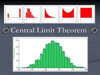
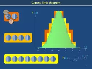
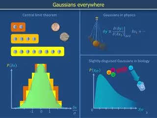
Central Limit Theorem • When dealing with a statistic that uses a sum of some sort we can theoretically show what the sampling distribution will be like through the Central Limit Theorem
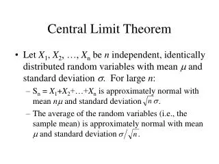
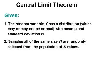
The central limit theorem • Take many random samples with replacement from a box model, all of the samples of size n. When n is sufficiently large, the distribution of the sample average (or sample %) is well-described by a normal curve • The mean of this normal curve is the EV and the standard deviation for this normal curve is the SE
The Central Limit Theorem • What does the CLT give us? A ton of stuff • We can find probabilities and percentiles using the the normal table • Can predict fairly accurately how unlikely it is to sample an observed sample mean • Can assess rather accurately how likely a population mean lies within an interval
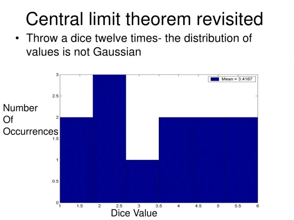
Central Limit Theorem • What happens if the distribution of the original variable is not symmetric (or think about the distribution of the values on the tickets in a box) • The central limit theorem still kicks in (the sample size n just needs to be bigger) • What happens if the distribution of the original variable is bimodal • The central limit theorem still kicks in (the sample size n just needs to be bigger) • This is absolutely a fantastic result !!!
Does CLT apply • A box consists of 9 ones and 1 zero. A random sample of size 50 is drawn with replacement from the box and the number of ones are counted. • A box consists of the ages of the 100 students in our stat class (assume that the mean is 20 and sd is 1). A random sample of size 50 is drawn with replacement from the box and and the 25th percentile is computed.
Central Limit Theorem M&Ms • Pick 50 M&Ms at random (from a bag). • How likely is it to have less than 40% yellow and brown M&Ms in the bag? • Assume 50% of all M&M’s are yellow and brown (source: M&M’s home page) • For a sample proportion of yellow and brown M&Ms • EV = 0.5 and SE =
Size of sample • For binomial (categorical data with two categories) data, the CLT usually kicks in pretty well when both of the following conditions on sample size are met
CLT and M&Ms • Since n=50, CLT applies • The probability of getting less than 40% yellow and brown M&Ms in a bag of 50 is • It is somewhat unusual to get less than 40% yellow and brown M&Ms (about 8 chances in 100)
CLT household example • The average size of U.S. households is 2.6 people. The SD of household size is 1.42. (These are true values from the U.S. Census). • Pick 200 houses at random in the U.S. • How likely is it that we’ll get a sample average household size of 3 or more?
CLT household example • For a sample average of 200 households • EV = 2.6 and SE = • The chance of getting an average household size greater than 3 equals the area under the standard normal curve to the right of 4. This is a very small chance
Alumni donations example • In a random sample of 100 alumni, what is the chance that more than half donated?
Alumni donations example • What is the chance that the sample average of donations from 100 randomly picked alumni will be between $50 and $100
CLT under three conditions • If original variable follows a normal distribution no need for CLT. We know the sampling distribution of a sum theoretically • If distribution of original variable is symmetric and unimodal then CLT holds for a small sample size (say less than 15) • If distribution is skewed, not unimodal then the CLT holds after a larger sample size • how large depends on the sharpness of the skew. In this class we will follow convention and say 30.
Parameter μ Inference Statistic Sample


