Download
1 / 36
610 likes | 1.24k Vues
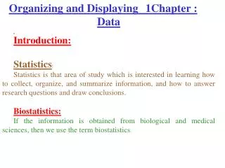
1 Chapter : Organizing and Displaying Data Introduction: Statistics : Statistics is that area of study which is interested in learning how to collect, organize, and summarize information, and how to answer research questions and draw conclusions. Biostatistics:

E N D
1Chapter : Organizing and Displaying Data Introduction: Statistics: Statistics is that area of study which is interested in learning how to collect, organize, and summarize information, and how to answer research questions and draw conclusions. Biostatistics: If the information is obtained from biological and medical sciences, then we use the term biostatistics.
Populations: A population is the largest group of people or things in which we are interested at a particular time and about which we want to make some statements or conclusions. Samples: From the population, we select various elements (or individuals) on which we collect our information. This part of the population on which we collect data is called the sample. Sample Size: The number of elements in the sample is called the sample size and is denoted by n. Variables: The characteristics to be measured on the elements of the population or sample are called variables.
Variables: The characteristics to be measured on the elements of the population or sample are called variables. Example of variables: - Height - no. of cars - sex - educational level
Types of Variables: (1) Quantitative Variables: The values of a quantitative variable are numbers indicating how much or how many of something. Examples: - height - family size - age
(2) Qualitative Variables: The value of a qualitative variable are words or attributes indicating to which category an element of the population belong. Examples: - blood type - educational level - nationality
Types of Quantative Variables: • Discrete Variables: • A discrete variable can have only countable number of values • Examples: • Family size (x = 0, 1, 2, 3, … ) • Number of patients (x = 0, 1, 2, 3, … )
Continuous Variables: A continuous variable can have any value within a certain interval of values. Examples: - height (140 < x < 190) - blood sugar level (10 < x < 15)
Variable Quantitative Qualitative Discrete Continuous
1.2.Organizing The Data Ungrouped (or Simple) frequency distributions : Used for: · -qualitative variables · -discrete quantitative variables with a few different values - Grouped frequency distributions : Used for: · - continuous quantitative variables · - discrete quantitative variables with large number of different values
Example: (Simple frequency distribution or ungrouped frequency distribution). The following data represent the number of children of 16 Saudi women: 3, 5, 2, 4, 0, 1, 3, 5, 2, 3, 2, 3, 3, 2, 4, 1 - Variable = X = no. of children (discrete, quantitative) - Sample size = n = 16 - The possible values of the variableare: 0, 1, 2, 3, 4, 5
no. of children (variable) Frequency (no. of women) Percentage Freq. (= R.F. * 100%) Relative Freq. (R. F.) (=Freq /n) 1 0.0625 6.25% 0 12.5% 1 2 0.125 0.25 2 4 25% 3 5 0.3125 31.25% 12.5% 4 2 0.125 12.5% 5 2 0.125 100% 1.00 Total n=16 Simple frequency distribution of the no. of children Note Total of the frequencies = n = e sample sizeTh ·Relative frequency = frequency/n Percentage frequency = Relative frequency *100%
· Frequency bar chart is a graphical representation for the simple frequency distribution.
17.0 17.7 15.9 15.2 16.2 17.1 15.7 17.3 13.5 16.3 14.4 15.8 15.3 16.4 13.7 16.2 16.4 16.1 17.0 15.9 14.0 16.2 16.4 14.9 17.8 16.1 15.5 18.3 15.8 16.7 15.9 15.3 13.9 16.8 15.9 16.3 17.4 15.0 17.5 16.1 14.2 16.1 15.7 15.1 17.4 16.5 14.4 16.3 17.3 15.8 Example 1.2: (grouped frequency distribution) The following table gives the hemoglobin level (g/dl) of a sample of 50 men. - Variable =X= hemoglobin level (continuous, quantitative) - Sample size = n = 50 - Max= 18.3 - Min= 13.5
Class Interval (Hemoglobin level) Frequency (no. of men) Cumulative Relative Frequency Relative Frequency Cumulative Frequency 13.0 - 13.9 14.0 - 14.9 15.0 - 15.9 16.0 - 16.9 17.0 - 17.9 18.0 - 18.9 3 5 15 16 10 1 0.06 0.10 0.30 0.32 0.20 0.02 3 8 23 39 49 50 = n 0.06 0.16 0.46 0.78 0.98 1.00 Total n=50 1.00 50 menGrouped frequency distribution for the hemoglobin level of the Notes · class interval = C. I. · Cumulative frequency of a class interval = no. of values (frequency) obtained in that class interval or before. Mid-Point (Class Mark) of C. I =
Class Interval True C. I. Class mid-point frequency 13.0 - 13.9 14.0 - 14.9 15.0 - 15.9 16.0 - 16.9 17.0 - 17.9 18.0 - 18.9 12.95 - 13.95 13.95 - 14.95 14.95 - 15.95 15.95 - 16.95 16.95 - 17.95 17.95 - 18.95 (13.0+13.9)/2 = 13.45 (14.9+14.9)/2 = 14.45 15.45 16.45 17.45 18.45 3 5 15 16 10 1 lower upper True True limits limits lower upper (L.L) (U.L.) limits limits
Displaying grouped frequency distributions: • For representing frequency or relative frequency distributions, we have • The following graphical presentations: • Histograms • Polygon • Curves
For representing cumulative frequency or cumulative relative frequency distributions: • · Cumulative Curves • · Cumulative Polygon (ogives)