Simulation Model for Input Optics Impact Analysis on Ground Motion in LIGO
This study presents a simulation model aimed at analyzing the effects of ground motion on the input optics and beam in the LIGO observatory. The objectives include building an Input Optics (IO) box using E2E, integrating it with SimLIGO, and conducting simulations with real-time ground motion data. The method involves creating a Small Optic Suspension (SOS) box, validating its performance, and using it to damp motion on optics. Preliminary results demonstrate effective local damping optimization and integration of the Mode Cleaner with the interferometer framework.

Simulation Model for Input Optics Impact Analysis on Ground Motion in LIGO
E N D
Presentation Transcript
Modeling the Input Optics using E2E R. Dodda, T. Findley, N. Jamal , K.Rogillio, and S. Yoshida, Southeastern Louisiana University – Acknowledgement – LIGO Livingston Observatory, SURF 2004, NSF B. Bhawal, M. Evans, V. Sannibale, and H. Yamamoto
Objectives A simulation model will be very convenient to study the impact of ground motion on the input optics, and on the input beam. Therefore, we seek to do the following: 1. Build an IO box using E2E ( time domain). 2. Integrate it with the Simligo. 3. Run simulation with real-time ground motion.
The Process 1. Make a Small Optic Suspension (SOS) box, and validate it. 2. Use the SOS box to damp the motion of an optic when real-time ground motion is given. 3. Create a Mode Cleaner (MC) box, and try to lock the cavity when real-time ground motion is given to the Mode Cleaner optics. 4. Put all the optics ( MCs, SM, and MMTs ) in order, and create the Input Optic (IO) box. 5. Use the IO box in Simligo, and run the simulation for the entire detector.
Validating SOS – Role of the Table Top motion MC1 Yaw motion using two different schemes Schematic diagram of the SOS box with HAM motion as input
V òò ACCX dt dt HAM table U q Vibration isolation stacks u v ¶ ¶ 1 1 - = - Table yaw = ( ) { ik u ( y , t ) ik v ( x , t )} 1 2 Accelerometer ¶ ¶ 2 y x 2 w ± w ± ( ) ( ) i t k y i t k x = = u ( y , t ) A e , v ( x , t ) A e 1 1 2 2 0 0 = = w q = w - k k k ( ) i k ( ){ u ( y , t ) v ( x , t )} 1 2 Calculating the HAM table’s yaw X in Table u HAM stack box Table v Y in
SM (0.75, 0.45) V MMT1 (0.1, 0.4) MC3 (0.75, -0.05) U (0, 0) q MMT3 (-0.8, 0.6) MC1 (0.75, -0.25) Calculating the suspension point motions of the optics u(x,y)= U - yq v(x,y)= V + xq U: table’s center of mass translational motion V: table’s center of mass translational motion q: table’s yaw motion
Conclusions • HAM table motion estimated from the ACC[XY] DAQ signal • MC1, MC3 local damping optimized • MC box constructed and being tested • Combination of MC and IFO in progress