Download
1 / 37
380 likes | 512 Vues
Evaluating surface ozone-temperature relationships over the eastern U.S. in chemistry-climate models. D.J. Rasmussen, Arlene Fiore, Vaishali Naik , Larry Horowitz (GFDL/NOAA), Sean McGinnis (Princeton), and Martin Schultz ( Forschungszentrum Jülich ). A GFDL Lunchtime S eminar

E N D
Evaluating surface ozone-temperature relationships over the eastern U.S. in chemistry-climate models D.J. Rasmussen, Arlene Fiore, VaishaliNaik, Larry Horowitz (GFDL/NOAA), Sean McGinnis(Princeton), and Martin Schultz (ForschungszentrumJülich) A GFDL Lunchtime Seminar August 17th, 2011
The U.S. O3 problem: over 150 million people breathe air deemed unhealthy by EPA The 8-hour O3 standard is 0.075ppm (~ 75ppb) [EPA, 2010] About 1 in 2 people in the U.S. live in these areas (*) To attain this standard: the 3-year average of the fourth-highest daily maximum 8-hour average ozone concentrations measured at each monitor within an area over each year must not exceed 0.075 ppm. (effective May 27, 2008)
Presentation Outline • Implications for air quality response to climate change • Characterizing the O3-temperature relationship over the eastern US • How well does a chemistry-climate model represent this relationship, particularly in light of a modeled summertime O3 bias over this region? • Do biases in surface temperature contribute to this modeled O3 bias?
Surface O3 varies strongly with temperature Observational studies have shown strong correlation between surface temperature and O3concentrations (Bloomer et al., 2009; Camalier et al., 2007; Cardelino and Chameides, 1990; Clark and Karl, 1982; Korsog and Wolff, 1991) Observations U.S. EPA CASTNet c/o A.M. Fiore Year-to-year temperatures have been observed to be strongly correlated with ozone Strong relationship between weather and pollution implies that changes in climate will influence air quality
Severe O3 pollution events associated with air stagnation in Europe 8-hr O3exceedances of 90 ppbv, summer 2003 Stagnant high pressure system over Europe (500 hPageopotential anomaly relative to 1979-1995 for 2-14 August, NCEP) # of Days 0-1 1-5 6-10 >10 H [ETC/ACC, CHMI] Correlation between surface O3 and temperature is strongly associated with air stagnation
What does a warming planet imply for surface O3 in the eastern US? MDA8 O3(ppb) Changes in summer 8-h avg. daily maximum ozone from 2000-2050 climate change eastern US Temperature (K) [IPCC, AR4, Ch. 11] [Wu et al., 2008] Higher temperatures, stagnation • Models agree that 2000-2050 climate change will increase surface ozone most over polluted regions (3-5 ppb). • Most models find climate change will exacerbate pollutionepisodes (up to 10 ppb) due to increased stagnation and higher temperatures. • Models fairly robust in simulating O3 increases in Northeast and Midwest U.S.
Current generation global models northeastern US How accurate are these models at reproducing observed seasonal O3 concentrations? Surface Ozone (ppb) Obs. = black Ensemble mean/median = red/blue • A pervasive high summertime O3 bias exists across both eastern US regions [A.M. Fiore, L.W. Horowitz et al., 2009; Murazaki and Hess, 2006; Reidmiller et al., 2009] • These biases raise concern of the ability of chemistry-climate models to project accurately the response of air pollution to climate change southeastern US Surface Ozone (ppb)
Motivating Questions • 1) Can we characterize long-term O3 response to year-to-year temperatures for regions over the eastern US for purposes of chemistry-climate model evaluation? • 2) Despite a known modeled ozone bias, can the GFDL AM3 chemistry-climate model represent the responseof surface O3 to interannual variations in temperature? • 3) Do modeled temperature biases contribute to these modeled ozone biases? • We hypothesize that: • Adequate representation of observed, climatological O3-temperature relationships will help to build confidence in future projections of the air quality response to changes in climate
Representing the O3 – temperature relationship • We use temperature as a proxy to synthesize the complex effects of meteorological and chemical factors influencing O3 concentrations • We represent these aggregate effects as a total derivative, • The O3-temperature relationship is thought to represent at least three components in the eastern US: [Jacob et al., 1993; Olszyna et al., 1997] [Meleux et al., 2007; Guenther et al., 2006] [Sillman and Samson, 1995] • meteorology • chemistry • emissions
Over what range of temperatures does O3 increase? Ozone’s relationship with temperature is non-linear, but it has been observed to be linear for ranges of temperatures… Cleveland, OH Camalier, 2007 Log O3 (ppb) Max. 1 hr. O3 (ppb) South Coast Air Basin, CA 280 290 300 Tmax (K) [Camalier et al., 2007] Tmax (K) [Steiner et al., 2010] O3 found to typically increase linearly between 290-305 K [Bloomer et al., 2009; Camalier et al., 2007; Sillman and Samson, 1995; Steiner et al., 2010]
Observation network EPA CASTNet sites used and locations: co-located meteorological and chemical observations Observations: EPA Clean Air Status and Trends Network (CASTNet; designed for measurements to be representative of the regional scale) Most sites have record lengths spanning 1988-2009
statistical approach to the O3-temp relationship We focus on the warm season over the eastern US where O3 and temperature are well correlated [Dawson et al., 2007; Lin et al., 2001; Sillman and Samson, 1995] We use maximum daily 8-hour average (MDA8) O3 and maximum daily surface temperature (Tmax) to focus on the daytime (deep, well-mixed, boundary layer) units = ppb O3 per oC/ K
Humans can influence O3 sensitivity to temperature by changing the O3 production chemistry CO VOC NOx+ Sunlight = O3 1999 NOx State Implementation Plan (SIP) Call National Ozone Season NOx Emissions from Power Plants NOx (million tons/ 5 months) 43% decrease in eastern US NOx emissions! [c/o US EPA] Changes to anthropogenic NOx emissions have a substantial effect on the sensitivity of O3 to temperature
effects of NOx emission controls on O3sensitivity 95% 75% 50% 25% 5% Great Lakes (May-October) Great Lakes Pre 2002: 3.1 ppb O3 K-1 Post 2002: 2.1 ppb O3 K-1 1 ppb O3 K-1 decrease 20 25 30 35 Temperature (C) [Bloomer et al., 2009] • ∆ NOxemissions decreased ozone levels over the entire distribution • The ozone sensitivities to temperature also decreased across the distribution • Different statistical methods reveal the same 1 ppb O3 K-1 decrease during O3 season
AM3 simulations • We use a 20-year (1981—2000) run of the GFDL AM3 CCM [Donner et al., 2011; Naik et al., in prep] • Interactive isoprene (responds to solar radiation and temperature) (MEGAN) following that used in MOZART-4 [Emmons et al., 2010] • Forcings: • Observed SSTs and sea ice [Rayner et al., 2003] • ACCMIP aerosol and O3 precursor emissions (as used in CM3 CMIP5 simulations) [Lamarqueet al., 2010] Little to no change in eastern US NOx emissions in model run
“climatological” O3-temperature relationships correlating MDA8 O3 and daily Tmax July CASTNet correlation (r) 1988-1999 1981-2000 July O3 is well correlated with Tmax correlations too low in southern US -problem representing inflow of marine air, convective ventilation, isoprene chemistry in this region?
“climatological” O3-temperature relationships July CASTNet slope (ppb K-1) 1988-1999 1981-2000 mO3-Ttoo low July mO3-T highest in Mid-Atlantic and southern US GFDL AM3 produces range of mO3-T over Northeast and portions of the Great Lakes Remains unclear why GFDL AM3 struggles in Mid-Atlantic and southern US
Regional approach to characterizing O3-temperature relationships We group CASTNet sites into chemically and meteorologically coherent regions Motivated by past statistical analyses [Bloomer et al., 2009; Eder et al., 1993; Lehman et al., 2004]
Regional approach: Northeast CASTNet sites We average over all CASTNet sites to isolate the regional response of O3 to temperature
Regional approach: Northeast Large standard errors highlight the need for longer datasets = regional avg. of MDA8 O3 and Tmax; each point is data from one year highest O3 sensitivities to temperature in summer (4-5 ppb O3K-1) r2 = .28 mO3-T = 4 ppb O3 K-1
Regional approach: Northeast Tmax is well simulated +10-15 ppb modeled MDA8 O3 bias CASTNet: r2 = .3, m = 4 ppb O3 K-1 GFDL AM3: r2 = .4, m = 4 ppb O3K-1 Despite the presence of excess modeled MDA8 O3… MDA8 O3 sensitivity to year-to-year variations in Tmax are reproduced by GFDL AM3 in the Northeast
Regional approach: Mid-Atlantic Again, we average over all CASTNet sites to isolate the regional response of O3 to temperature
Regional approach: Mid-Atlantic Highest O3 sensitivities to temperature are in summer (4-6 ppb O3 K-1) r2 = .26 mO3-T = 6 ppb O3 K-1
Regional approach: Mid-Atlantic Modeled Tmaxare too large 10-30 ppb modeled O3bias CASTNet: r2 = .3, m = 6 ppb O3 K-1 GFDL AM3: r2 = .6, m = 2 ppb O3 K-1 model slopes are ~4 ppb O3 K-1 too low in the summer months What effect does Tmax bias have on O3 over the eastern US?
Modeled tmax bias and O3sensitivity multiply Tmax biases by mean regional sensitivity of 3 ppb O3 K-1 JUN JUL AUG SEP Maurer et al. [2002] NARR Tmaxbiases are responsible for up to 10-15 ppbof the summer O3 bias, specifically in the interior of the Mid-Atlantic region • cannot be the major driver of the large-scale O3 bias
Conclusions Despite modeled O3 biases, the GFDL AM3 reproduces mO3-T in the Northeast, although it underestimates mO3-T by 2–4 ppb K-1 in the summer over the Mid-Atlantic • model skill at simulating fundamental meteorological processes may be contributing to the inaccuracies in producing mO3-T over the Mid-Atlantic • We estimate a maximum contribution of 10–15 ppb MDA8 O3from simulated Tmax biases over the Mid-Atlantic • We find modeled (+) Tmax biases are not the major driver of the large-scale excess modeled O3
evaluating modeled diurnal temperature and O3 When diurnal temperature biases are highest, are the O3 biases correspondingly highest?
Why does the model struggle in the southeastern US? cyclonic ventilation of the eastern U.S. Fundamentally different meteorological processes modulate O3 levels in the southern and northern halves of the eastern US: • In the Northeast: pollutant ventilation is known to be driven by migratory cyclones associated with cold fronts [Leibensperger et al., 2008; Logan, 1989, Vukovich, 1995] • In the Southeast: Deep convection and inflow from the Gulf of Mexico are known to ventilate O3 in the boundary layer [Li et al., 2005] • The skill of the GFDL AM3 chemistry-climate model in simulating these meteorological processes may be help explain why O3-temp sensitivities are not accurately produced
GFDL AM3 CCM eastern U.S. summertime O3 bias • GFDL AM3 CCM has a high O3 bias in summer months in the eastern U.S. [10-30 ppb] June monthly mean MDA8 O3 Bias (GFDL minus CASTNet)
Spatial distribution of NA tropospheric NO2 SCIAMACHY data. May-Oct 2004 [R.V. Martin, Dalhousie U.]
Biogenic VOC (isoprene) column measurements Millet et al. [2008]
Emissions of VOCs spatially vary Switches polluted areas in U.S. from NOx-saturated to NOx-limited regime! recognized in Revised Clean Air Act of 1999 Anthropogenic VOCs Isoprene (biogenic VOC) Jacob et al., J. Geophys. Res. [1993]
(1) Regional stagnation/ ventilation Degree of mixing strong mixing Boundary layer depth pollutant sources cyclonic ventilation of the eastern U.S. [Manhattan, NY]
(3) Emissions (biogenic depend strongly on temperature) VOCs T (2) PAN chemistry, (3) biogenic emissions (2) the amount of NOx (NO+NO2) sequestered by peroxyacetylnitrate (PAN) decreases with increasing temperature
Why is O3 relevant to climate? Increasing… Effect on O3 concentrations: Stagnation Temperature Wind speed Mixing depth Cloud cover Humidity = = [Jacob and Winner, 2009]
Ozone (O3) in the atmosphere Good (UV shield) 90% of column O3 in our atmosphere exists here in the stratosphere Stratosphere Troposphere Bad (Smog) surface O3 is toxic to both people and plants