Download

1 / 38
400 likes | 615 Vues
Decadal Variability, Impact, and Prediction of the Kuroshio Extension System . B. Qiu 1 , S. Chen 1 , N. Schneider 1 and B. Taguchi 2 1. Dept of Oceanography, University of Hawaii, USA 2. Earth Simulator Center, JAMSTEC, Japan.

E N D
Decadal Variability, Impact, and Prediction of the Kuroshio Extension System B. Qiu1, S. Chen1, N. Schneider1 and B. Taguchi2 1. Dept of Oceanography, University of Hawaii, USA 2. Earth Simulator Center, JAMSTEC, Japan Climate Implications of Frontal Scale Air-Sea Interaction Workshop, Boulder, 5-7 August 2013
Outlines • Observed decadal changes in the Kuroshio Extension system • Forced vs. intrinsic KE variability and impact on SST front • KE index and its prediction AVISO satellite altimeter data: 10/1992-present
Mesoscale eddy fluctuations Low-frequency circulation modulations
Altimeter-derived KE paths: Oscillations between stable and unstable states
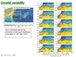
Altimeter-derived KE paths: Oscillations between stable and unstable states Stable yrs: 1993-94, 2002-04, 2010-2013 Unstable yrs: 1996-2001, 2006-08
Yearly-averaged SSH field in the region surrounding the KE system
Various dynamic properties representing the decadal KE variability
Various dynamic properties representing the decadal KE variability Question 1:What causes the transitions between the stable and unstable dynamic states of the KE system?
Decadal KE variability lags the PDO index by 4 yrs ( r=0.67 ) • Center of wind forcing is in eastern half of North Pacific basin • + PDO generates negative local SSHAs through Ekman divergence, and vice versa
KE <∂h> SSH field SSHA along 34°N PDO index H L H L 135E 145E 155E 165E center of PDO forcing
SSHA along 34°N PDO index/AL pressure SSH variability vs wind forcing • Large-scale SSH changes are governing by linear vorticity dynamics: H L • Given the wind forcing, SSH changes can be found along the Rossby wave paths: H L cR: observed value wind stress: NCEP reanalysis center of PDO forcing
Wind-forced SSHA along 34°N SSHA along 34°N PDO index/AL pressure H L H L center of PDO forcing
KE strength of 142°-180°E (Taguchi et al. 2007) See also Nonakaet al. (2006), Pierini et al. (2009)
Question 2: What is the relative importance of the PDO-related wind forcing vs. the internal oceanic eddy forcing?
Quantifying wind- vs. eddy-forced KE variability in a 1.5-layer reduced-gravity North Pacific Ocean model • Governing equations: where is velocity vector and is upper layer thickness. • denotes the external wind forcing; given by interannually varying, or climatological, monthly NCEP data • denotes the oceanic eddy forcing; inferred from the weekly AVISO anomalous SSH data • North Pacific domain: 0°-50°N, 120°E-75°W • Horizontal eddy viscosity: Ah = 1,000 m2/s
Modeled KE properties wind forcing only Modeled KE properties clim. wind + eddy forcing Observed KE properties • Wind forcing (only) case underestimates KE position/intensity changes and misses eddy signals • Eddy + clim. wind forcing case fails to capture the decadal KE signals
Modeled KE properties wind + eddy forcing Modeled KE properties clim. wind + eddy forcing Observed KE properties • Combined forcing by time-varying wind and eddy flux divergence generates the observed, decadal modulations of the KE system
KE dynamic state affects regional SST and cross-front SST gradient
JF rms 850mb v’T’ of stormtrack variability (Nakamura et al. 2004) By carrying a significant amount of warm water from the tropics, KE is the region of intense air-sea interaction RMS SSH variability (>2yrs) JFM rms net surface heat flux variability
850mb v’T’ and Q’ regressed to the KE dynamic state in 1977-2012 JF rms 850mb v’T’ of stormtrack variability (Nakamura et al. 2004) JFM rms net surface heat flux variability When KE is stable, more heat release from O to A and a northward shift of stormtracks
Question 3: Can the decadally-modulating KE dynamic state be predicted in advance?
A composite index quantifying the KE dynamic state: the KE index KE index : average of the 4 dynamic properties (normalized)
Regression between the KE index and the AVISO SSH anomaly field KE index: represented well by SSH anomalies in 31-36°N, 140-165°E Implications: Predicting KE index becomes equivalent to predicting SSH anomalies in this key box
1. Prediction with Rossby wave dynamics KE index and x-t SSHAs h1(x, t) = hobs [ x+cR(t-t0), t0 ] where hobs(x, t0): initial SSHAs cR: Rossby wave speed The basis for long-term KE index prediction rests on 2 processes: 1. Oceanic adjustment in mid-latitude North Pacific is via slow, baroclinic Rossby waves
Mean square skill of the predicted KE index • Compared to damped persistence, wave-carried SSHAs increase predictive skill with a 2~3 yr lead (Schneider and Miller 2001)
NCEP mean wind stress curl field The basis for long-term KE index prediction rests on 2 processes: 2. The KE decadal variability affects the basin-scale wind stress curl field stormtracks KEI>0 KE index-regressed curl field (tropical influence removed)
Other studies of wind stress curl responses to KE variability NCEP mean wind stress curl field KE index-regressed curl field (tropical influence removed)
The reason behind enhanced predictive skill with the 4~6 yr lead: delayed negative feedback mechanism wind curl > 0 SSHA < 0 wind curl > 0 SSHA < 0 stormtracks KEI>0 SSHA < 0 RW propagation KEI>0 half of the oscillation cycle: ~5 yrs in the N Pacific basin
1. Prediction with Rossby wave dynamics KE index and x-t SSHAs h1(x, t) = hobs [ x+cR(t-t0), t0 ] where hobs(x, t0): initial SSHAs cR: Rossby wave speed 2. Prediction with Rossby wave dynamics + KE feedback to wind forcing h2(x, t) = h1(x, t) + ∫ b[ x+cR(t’-t0) ] K(t’) dt’ t t0 where b(x): feedback coefficient K(t): forecast KE index
Mean square skill of the predicted KE index • Compared to damped persistence, wave-carried SSHAs increase predictive skill with a 2~3 yr lead (Schneider and Miller 2001) • Additional skill is gained with the 4~6 yr lead by considering the wind forcing due to KE feedback
Summary • KE dynamic state (i.e. EKE level, path, and jet/RG strengths) is dominated by decadal variations. It impacts the broad-scale cross-front SST gradient. • SSH anomaly signals in 31-36°N, 140-165°E provide a good proxy for the decadally-varying KE index. • A positive KE index induces overlying-high and downstream- low pressure anomalies. This feedback favors a coupled mode with a ~10 yr timescale. • Oscillatory nature of this mode enhances predictability • Compared to Rossbywave dynamics, inclusion of the KE-feedback wind forcing increases predictive skill with a lead time from 2~3 to 4~5 yrs. • Due to the persistent negative PDO phase, a prolonged stable KE dynamic state (until 2017) is predicted.
2013-2023 KE index forecast based on 2012 AVISO SSH data • KE dynamic state (i.e. EKE level, path, and jet/RG strengths) is dominated by decadal variations. It impacts the broad-scale cross-front SST gradient. • SSH anomaly signals in 31-36°N, 140-165°E provide a good proxy for the decadally-varying KE index. • A positive KE index induces overlying-high and downstream- low pressure anomalies. This feedback favors a coupled mode with a ~10 yr timescale. • Oscillatory nature of this mode enhances predictability • Compared to Rossbywave dynamics, inclusion of the KE-feedback wind forcing increases predictive skill with a lead time from 2~3 to 4~5 yrs. • Due to the persistent negative PDO phase, a prolonged stable KE dynamic state (until 2017) is predicted.
Yearly SSH anomaly field in the North Pacific Ocean + + - - - + / : PDO index
Schematic of the decadally-modulating Kuroshio Extension system Stable Dynamic State + PDO • Ekman divergence in the east • Incoming negative SSHA • Weakening RG and southerly KE jet • Enhancing local EKE level • Eddy-eddy interaction re-enhances the RG • Reducing EKE level • Strengthening RG and northerly KE jet • Incoming positive SSHA • Ekmanconver-gence in the east Unstable Dynamic State – PDO N.B. Nonlinearity important; phase changes paced by external wind forcing
Bimodal decadal KE variability can be purely nonlinearly driven Pierini et al. (2009, JPO)