Download
1 / 40
410 likes | 1.11k Vues
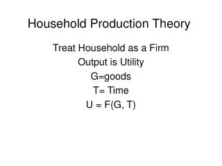
Household Production Model I:. The allocation of time. Household production model. In the household production model, utility is derived from the activities (Z i ) in which people are engaged. U=U(Z 1 , Z 2 ,…, Z N )

E N D
Household Production Model I: The allocation of time
Household production model • In the household production model, utility is derived from the activities (Zi) in which people are engaged. • U=U(Z1, Z2,…, ZN) • Each final commodity is produced and consumed within the household by combining time and purchased inputs.
Example: college attendance • College attendance • Requires time as well as purchased inputs (tuition, books, supplies, etc.)
Full cost • The full cost of an activity includes the opportunity cost of time as well as the opportunity cost of purchased inputs. • Example – college enrollments often increase during recessions due to lower opportunity cost of time.
Assumptions • U=U(Z1, Z2,…, ZN) • Zi=fi(ti,xi) • Where: • ti = amount of time devoted to producing and consuming commodity i. • xi = amount of purchased inputs devoted to producing and consuming commodity i. (This is a composite commodity that is an index of all purchased inputs used in producing final commodities.)
Constraints Solving the time constraint for time at work: Substituting this into the goods constraint results in:
Full-income constraint • After a little algebraic manipulation, the full income constraint is given by the formula below. • The first time is the opportunity cost of goods, the second is the opportunity cost of time.
Full-income constraint (cont.) • The full-income constraint may also be expressed as: • Where FCi = full cost of Zi:
Applications • Individuals are assumed to minimize the full cost of consuming any commodity. This model may explain: • the growth of the fast-food industry, • why convenience stores can survive while charging higher prices than grocery stores, • the decline in fertility, and • why many people do not use coupons in grocery stores.
Isoquants • This diagram illustrates the possible combinations of time and purchased inputs to provide a given quantity and quality of meals.
Indifference curves / isoquants • An isoquant is also an indifference curve since Zi is held constant.
Points on an isoquant • At point A, an individual may prepare meals using basic ingredients such as flour, vegetables, meat, etc. • the individual is using a large quantity of time, but a relatively low level of purchased inputs.
Points on an isoquant (cont.) • At point B, the individual prepares meals of the same quality using prepackaged mixes, frozen meals, and other preprocessed ingredients.
Points on an isoquant (cont.) • The individual uses less of his or her own time and more purchased ingredients when producing and consuming meals at point C. • This may involve meals consumed in restaurants or meals delivered to the home from restaurants.
Other isoquants • Points that lie above an isoquant correspond to the production of a higher level of Zi.
Isocost curves • Isocost curves have a slope equal to -w/p (the negative of the real wage). • The level of total costs increase as the level of time and purchased inputs increase.
Cost minimization • The least costly combination of time and purchased inputs occurs at the point of tangency between the isoquant curve and an isocost curve. • This occurs at point E.
Wage increase: substitution effects • First type: • As the wage rate increases, the relative price of time rises and households substitute purchased inputs for time in the production and consumption of a given level of each commodity.
Substitution effects • Second type: • Some activities are inherently more time-intensive than other activities. When the wage rate increases, the relative price of time-intensive activities increases. In response, goods-intensive activities are substituted for time-intensive activities. • Under both types of substitution effect, a higher wage reduces the quantity of time used in household production and increases the amount of time spent at work.
Income effect • An increase in the wagealso increases the quantity of final commodities (Zi) consumed. • This income effect tends to increase the amount of time required for the production and consumption of these commodities. x C x B t t B C
Backward-bending labor supply curve • The labor supply curve is upward sloping if the substitution effects are larger in magnitude than the income effect. • An individual operates on a backward-bending portion of his or her labor supply curve if the income effect is larger than the substitution effects.
Specialization • If a household wishes to produce output efficiently, each individual should specialize in those tasks in which he or she possesses a comparative advantage. • a household member possesses a comparative advantage in an activity if the opportunity cost of the activity is lower for this individual than for any other member of the household.)
Sources of comparative advantage • A comparative advantage may exist if: • an individual is more productive in an activity than other members of the household (in this case an “absolute advantage” is said to occur), or • because the individual’s time is relatively less valuable in alternative activities.
Gender division of labor • Historically, married women have tended to specialize in household production and married males have tended to specialize in market production. • Comparative advantage for women in household production in the past? • Possible reasons: • high completed fertility rates, • high infant mortality rates, and • labor market discrimination.
Evolving gender roles • As infant mortality and completed fertility rates decline and as female wage rates rise, it is expected that this division of labor between spouses will be altered. • In recent years, married women have substantially increased the amount of time spent in the paid labor market and have spent slightly less in household production). • Married men now spend slightly more time in household production than in the past.
Specialization or shared activities? • Both spouses will tend to work together in household production tasks in which their time is complementary • Individuals will specialize (according to comparative advantage) when one spouse’s time is a substitute for that of the other spouse.
Additional worker effect • The labor force participation rate generally declines during recessions as a result of an increase in the number of discouraged workers. • In a household, however, one spouse may increase his or her labor supply (or enter the labor market) if the other spouse becomes unemployed. • This “additional worker effect” partly offsets the “discouraged worker effect” discussed earlier. • The additional worker effect is smaller in magnitude than the discouraged worker effect.
Additional worker effect (cont.) • The additional worker effect is relatively small because the expected wage declines during a recession:E(w) = pw where: E(w) = expected wage p = probability of employment w = wage rate if employed As the unemployment rate rises during a recession, the probability of being employed, p, declines, leading to a reduction in the expected wage.
Female labor supply and divorce • Married women tend to increase their labor supply when a divorce becomes more likely. • This is partly to prepare for the reduction in the division of labor that occurs after the divorce. • Empirical evidence suggests that the level of per capita consumption declines by a larger amount in the portion of the splitoff household headed by divorced women.
Lifetime labor supply decisions • The productivity of time in the paid labor force varies over the lifecycle. • Market wages vary over time as productivity changes.
Lifecycle labor supply • individuals are expected to spend more time working in the paid labor market (and less time in household production) when market wage rates are relatively high.
Labor force participation and childrearing • Historically, many married females chose to reduce the quantity of labor supplied or leave the labor force during their childbearing years.
Changes in LFPR for married women • As fertility levels have declined and market wage rates have increased, a smaller proportion of married working mothers exit the labor force during the childbearing years today than in past decades.
Social Security & Retirement Age • an increase in the level of retirement benefits induces individuals to retire earlier.
Single-parent households and welfare • Many single parents (typically female) remain out of the labor force
Child Support Enforcement Act • the budget constraint facing the custodial parent shifts vertically upward. • reduces state welfare expenditures even if there is no effect on labor supply
Child Support Enforcement Act • Increases labor supply for some welfare recipients who were initially out of the labor force.
Child Support Enforcement Act • is expected to reduce labor supply if the custodial parent is initially working.