Newton’s Method: Solutions of Equations in One Variable
Learn about Newton’s Method for solving equations in mathematics using Taylor's expansion and iterative methods for convergence analysis.

Newton’s Method: Solutions of Equations in One Variable
E N D
Presentation Transcript
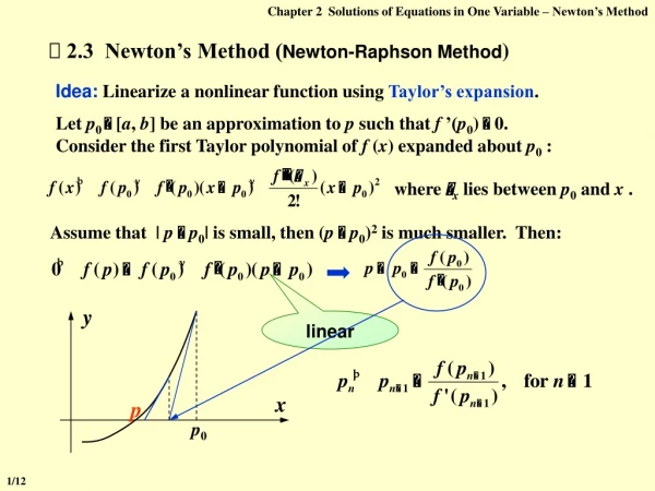
Chapter 2Solutions of Equations in One Variable – Newton’s Method where xlies between p0 and x . y x p p0 2.3 Newton’s Method (Newton-Raphson Method) Idea: Linearize a nonlinear function using Taylor’s expansion. Let p0 [a, b]be an approximation to p such that f ’(p0) 0. Consider the first Taylor polynomial off (x) expanded about p0 : Assume that | p p0| is small, then (p p0)2 is much smaller. Then: linear 1/12
Chapter 2Solutions of Equations in One Variable – Newton’s Method Proof: Newton’s method is just pn = g( pn – 1 ) for n 1 with f ’(p) 0 and is continuous f ’(x) 0 in a neighborhood of p g’(p) = g’(x) is small and is continuous in a neighborhood of p f ”(x) is continuous Theorem: Let f C2[a, b]. If p[a, b] is such that f(p) = 0 and f ’(p) 0, then there exists a > 0 such that Newton’s method generates a sequence { pn} (n = 1, 2, …) converging to p for any initial approximation p0 [p – , p + ]. a. Is g(x) continuous in a neighborhood of p? b. Is g’(x) bounded by 0 < k < 1in a neighborhood of p? g’(x) = 0 2/12
Chapter 2Solutions of Equations in One Variable – Newton’s Method | g(x) – p | < p0 p0 p0 Proof (continued): c. Does g(x) map [p – , p + ] into itself? = | g(x) – g(p) | = | g’() | | x – p | k| x – p | < | x – p | Note: The convergence of Newton’s method depends on the selection of the initial approximation. p 3/12
Chapter 2Solutions of Equations in One Variable – Newton’s Method p1 p0 Secant Method: What is wrong: Newton’s method requires f ’(x) at each approximation. Frequently, f ’(x) is far more difficult and needs more arithmetic operations to calculate than f(x). HW: p.75 #13 (b)(c), p.76 #15 secant line tangent line Slower than Newton’s Method and still requires a good initial approximation. tangentsecant Have to start with 2 initial approximations. 4/12
Chapter 2Solutions of Equations in One Variable – Newton’s Method Lab 02. Root of a Polynomial Time Limit: 1 second; Points: 3 A polynomial of degree n has the common form as Your task is to write a program to find a root of a given polynomial in a given interval. 5/12
Chapter 2Solutions of Equations in One Variable – Error Analysis for Iterative Methods Definition: Suppose { pn } ( n = 0, 1, 2, …) is a sequence that converges to p, with pn p for all n. If positive constants and exist with then { pn } ( n = 0, 1, 2, …) converges to p of order , with asymptotic error constant . 2.4 Error Analysis for Iterative Methods • If =1, the sequence is linearly convergent. • If =2, the sequence is quadratically convergent. The the value of , the faster the convergence. larger Q: What is the order of convergence for an iterative method with g’(p) 0? A: Linearly convergent. 6/12
Chapter 2Solutions of Equations in One Variable – Error Analysis for Iterative Methods This is a one line proof...if we start sufficiently far to the left. p n Q: What is the order of convergence for Newton’s method (where g’(p) = 0) ? Fast near a simple root. A: From Taylor’s expansion we have As long as f ’(p) 0, Newton’s method is at least quadratically convergent. Q: How can we practically determine and ? Theorem: Let p be a fixed point of g(x). If there exists some constant 2 such that g C [p – , p + ], g’(p) = … = g( – 1) (p) = 0, and g() (p) 0. Then the iterations with pn = g( pn – 1 ), n 1, is of order . 7/12
Chapter 2Solutions of Equations in One Variable – Error Analysis for Iterative Methods Newton’s method is just pn = g( pn – 1 ) for n 1 with It is convergent, but not quadratically. Q: What is the order of convergence for Newton’s method if the root is NOT simple ? A: If p is a root of f of multiplicity m, then f(x) = (x – p)mq(x) and q(x) 0. g’(p) = Q: Is there anyway to speed it up? A: Yes! Equivalently transform the multiple root of f into the simple root of another function, and then apply Newton’s method. 8/12
Chapter 2Solutions of Equations in One Variable – Error Analysis for Iterative Methods Let, then the multiple root of f = the simple root of . Apply Newton’s method to : Quadratic convergence Requires additional calculation of f ”(x); The denominator consists of the difference of two numbers that are both close to 0. HW: p.86 #11 9/12
Chapter 2Solutions of Equations in One Variable – Accelerating Convergence y y = g(x) y = x x p1 p p2 p0 2.5 Accelerating Convergence Aitken’s 2 Method: t(p1, p2) t(p0, p1) 10/12
Chapter 2Solutions of Equations in One Variable – Accelerating Convergence for n 0. Aitken’s 2 Method: Theorem: Suppose that { pn} (n = 1, 2, …) is a sequence that converges linearly to the limit p and that for all sufficiently large values of n we have ( pn – p)( pn+1 – p) > 0. Then the sequence { } (n = 1, 2, …) converges to p faster than { pn} (n = 1, 2, …) in the sense that Definition: For a given sequence { pn} (n = 1, 2, …), the forward differencepnis defined by pn= pn+1 – pn for n 0. Higher powers, kpn, are defined recursively by kpn = (k – 1pn ) for for k 2. Local quadratic convergence if g’(p) 1. Steffensen’s Method: 11/12
Chapter 2Solutions of Equations in One Variable – Accelerating Convergence Algorithm: Steffensen’s Acceleration Find a solution to x = g(x) given an initial approximation p0. Input: initial approximation p0; tolerance TOL; maximum number of iterations Nmax. Output: approximate solution x or message of failure. Step 1 Set i = 1; Step 2 While ( i Nmax) do steps 3-6 Step 3 Set p1 = g(p0) ; p2 = g(p1) ; p = p0 ( p1 p0 )2 / ( p2 2 p1 + p0 ) ; Step 4 If | p p0 | < TOL then Output (p); /* successful */ STOP; Step 5 Set i ++; Step 6 Set p0 = p ; /* update p0 */ Step 7 Output (The method failed after Nmax iterations); /* unsuccessful */ STOP. 12/12