Download
1 / 41
410 likes | 564 Vues
Modeling Peak Oil with the International Petroleum Production Model: IPPM.

E N D
Modeling Peak Oil with the International Petroleum Production Model: IPPM
“*This is a working document prepared by the Energy Information Administration (EIA) in order to solicit advice and comment on statistical matters from the American Statistical Association Committee on Energy Statistics. This topic will be discussed at EIA's spring 2008 meeting with the Committee to be held April 9, 2008.”
Overview • Concepts • Data assumptions • Methodology (model schematics) • Example output • Questions for the committee
Concepts • Peak oil • Oil streams • Regions • Assumptions
Peak Oil • The all time highest annual average production rate (million barrels per day, MMBD)
What is oil? Oil = Petroleum Liquids • Crude Oil & Lease Condensates • Natural Gas Plant Liquids (NGPL) • Extra-Heavy Crude Oil • Bitumen (oil sands) • Oil Shale (kerogen) • Crude Oil from Other Source Rock • Exclude: biofuels, CTL, GTL
Regional Groups • United States • Other non-OPEC • Middle East OPEC • Other OPEC • The model is expandable to many other regions or countries
Data and Assumptions (1) • World consumption path by t • World oil price by t • Initially In Place volumes (IIP) by r,s • Long term max Recovery Factors (RF) by r,s • Finding and Development costs (F&D) by r,s,cp • Lease and Operating costs by r,s • Taxes and Royalty rates by r,s • Cost of Capital by r,s Where r = region, s = stream, t = time, cp = cumulative production
Data and Assumptions (2) • Max production volumes by r,s,t • Max growth rates by r,s,t • Share of new production capacity added based on prior 1 to 10 year average versus economic profitability • Technology improvement rates by s,t • Allow negative profits (Y/N) • Number of annual supply increments up to 100 • Shape of Supply curves • Production profiles by r,s
Consumption Paths Note: Biofuels, gas-to-liquids, coal-to-liquids, and refinery gain are excluded
Initial-in-Place Estimates(trillion barrels) Sources: I.H.S. Energy, World Energy Council, USGS, Nehring Associates, EIA analysis Includes discovered and undiscovered volumes.
Recovery Factors • Recovery Factors • Typically vary between 10 to 70 percent • Increase with technology • Higher in “good” reservoirs
Model Schematic Below Ground “Candidate” Demand Scenarios Production Scheduling: Invest to create Proved Developed Reserves ? Above Ground • Proved developed reserves for different oil streams (conventional crude+condensate, NGPLs, bitumen, extra heavy oil, shale, and other source rock) are generated through investment, constrained by both above ground and below ground factors • The availability of production from proved developed reserves is used to assess the viability of “candidate” oil demand paths drawn from the recent U.S. Climate Change Science Program scenarios report.
Model Loop Loops through 2008 to 2200 five regions six streams
Scheduling: Investment In Incremental Production Capacity Potential Incremental Reserve Additions Cumulative Production plus Proved Developed Reserves Resource 1 Resource 2 Max RF1* IIP1 Max RF2* IIP2 Proved Developed Reserves (B) Proved Developed Reserves (B)
Capacity Addition Supply Curve Technology improvements shift the curve to the right. 65% of IIP
Petroleum Streams (and Regions) compete to provide Capacity Additions Crude oil Oil sands Oil sands become competitive with crude oil here. Volume
Example Output • The following charts are based on a middle consumption case • They illustrate how the model works
F&D Costs Market share constraints and different regional F&D costs prevent equilibration.
F&D Costs Here we see production constraints, combined with technology improvements push F&D costs down.
Questions for the committee • Is this approach appropriate for modeling long term industry behavior? • How might we better estimate • Recovery Factor improvements • Finding and Development cost evolution • Supply curve shape • Sensitivity analysis?
Next Steps • Refine IIP data sources • Better estimates of RF improvement • Supply curve refinement • Add environmental costs i.e. taxes
Thank you John Staub John.Staub@eia.doe.gov Tel: (773) 360-1942 Lauren Mayne Lauren.Mayne@eia.doe.gov Tel: (202) 586-3005 John Holte John.Holte@eia.doe.gov Tel: (202) 586-7818 www.eia.doe.gov