Download
1 / 45
450 likes | 602 Vues
RECOGNITION OF NONSTATIONARY SIGNALS. Joseph Picone, PhD Professor, Department of Electrical and Computer Engineering Mississippi State University. URL:. Engineering Terminology. Speech recognition is essentially an application of pattern recognition or machine learning to audio signals:

E N D
RECOGNITION OF NONSTATIONARY SIGNALS Joseph Picone, PhD Professor, Department of Electrical and Computer Engineering Mississippi State University URL:
Engineering Terminology • Speech recognition is essentially an application of pattern recognition or machine learning to audio signals: • Pattern Recognition: “The act of taking raw data and taking an action based on the category of the pattern.” • Machine Learning: The ability of a machine to improve its performance based on previous results. • A popular application of pattern recognition is the development of a functional mapping between inputs (observations) and desired outcomes or actions (classes). • For the past 30 years, statistical methods have dominated the fields of pattern recognition and machine learning. Unfortunately, these methods typically require large amounts of truth-marked data to be effective. • Generalization and Risk: There are many algorithms that produce very low error rates on small data sets, but many of these algorithms have trouble generalizing these results when constrained to limited amounts of training data., or encountering evaluation conditions different from the training data.
Fundamental Challenges: Generalization and Risk • Why research human language technology? • “Language is the preeminent trait of the human species.” • “I never met someone who wasn’t interested in language.” • “I decided to work on language because it seemed to be the hardest problem to solve.” • Some fundamental challenges: • Diversity of data, much of which defies simple mathematical descriptions or physical constraints (e.g., Internet data). • Too many unique problems to be solved (e.g., 6,000 language, billions of speakers, thousands of linguistic phenomena). • Generalization and risk are fundamental challenges (e.g., how much can we rely on sparse data sets to build high performance systems). • Underlying technology is applicable to many application domains: • Fatigue/stress detection, acoustic signatures (defense, homeland security); • EEG/EKG and many other biological signals (biomedical engineering); • Open source data mining, real-time event detection (national security). • Significant technology commercialization opportunities!
Fundamental Challenges in Spontaneous Speech • Common phrases experience significant reduction (e.g., “Did you get” becomes “jyuge”). • Approximately 12% of phonemes and 1% of syllables are deleted. • Robustness to missing data is a critical element of any system. • Linguistic phenomena such as coarticulation produce significant overlap in the feature space. • Decreasing classification error rate requires increasing the amount of linguistic context. • Modern systems condition acoustic probabilities using units ranging from phones to multiword phrases.
Speech Recognition Overview • Conversion of a 1D time series (sound pressure wave vs. time) to a symbolic description. • Exploits “domain” knowledge at each level of the hierarchy to constrain the search space and improve accuracy. • The exact location of symbols in the signal are unknown. • Segmentation, or location of the symbols, is done in a statistically optimal manner as part of the search process. • Complexity of the search space is exponential.
From a Signal to a Spectrogram • Convert a one-dimensional signal (sound pressure wave vs. time) to a time-frequency representation that better depicts the “signature” of a sound. • Use simple linear transforms such as a Fourier Transform to generate a “spectrogram” of the signal (spectral magnitude vs. time and frequency). • Key challenge: where do sounds begin and end in the signal?
From a Spectrum to Phonemes • The spectral signature of soundsvaries with its context (e.g., thereare 39 variants of “t” in English). • We use context-dependent modelsthat take into account the leftand right context (e.g., “k-ah+t”). • This unfortunately causes anexponential growth in the search space. • There are approx. 40 phones in English, and approx. 10,000 possible combinations of three phones, which we refer to as triphones. • Decision-tree clustering is used to reduce the number of parameters required to describe these models. • Since any phone can occur at any time, and any phone can follow any other phone, every frame of processing requires starting 10,000 new hypotheses. • Hence, to control complexity, the search is controlled using a top-down supervision (time-synchronous breadth-first search). • Less probable hypothesis are discarded each frame (beam search).
From Phonemes to Words • Phones are converted to words using a lexicon that typically contains between 100K and 1M words. • About 10% of the expected phonemes are deleted in conversational speech, so pronunciation models must be robust to missing data. • Many words have alternate pronunciations based on context, dialect, accent, speaking rate, etc. • Phoneme recognition accuracies are low (approx. 60%), but by using word-level supervision, recognition accuracy can be high (greater than 90%). • If any of 1M words can occur at almost any time, the size of the search space is enormous. Hence, efficient search strategies are critical, and only suboptimal solutions are feasible.
From Words to Concepts • Words can be converted to concepts or actions using various mapping functions (e.g., finite state machines, neural networks, formal languages). • Statistical models can be used, but these require large amounts of labeled data (word sequence and corresponding action). • Domain knowledge is used to limit the search space.
The Bayesian Approach to Speech Recognition InputSpeech • Based on a noisy communication channel model in which the intended message is corrupted by a sequence of noisy models • Bayesian approach is most common: • Objective: minimize word error rate by maximizing P(W|A) • P(A|W): Acoustic Model • P(W): Language Model • P(A): Evidence (ignored) • Acoustic models use hidden Markov models with Gaussian mixtures. • P(W) is estimated using probabilisticN-gram models. • Parameters can be trained using generative (ML)or discriminative (e.g., MMIE, MCE, or MPE) approaches. AcousticFront-end Research Focus Acoustic ModelsP(A/W) Language ModelP(W) Search Recognized Utterance
Towards Nonlinear Acoustic Modeling • ARHMM: • autoregressive time series model for feature vectors integrated into an HMM framework • GMMs: • use multiple mixture components to accommodate modalities in the data; • rely on a feature vector to capture dynamics of the signal; • classification tends to perform poorly on unseen data. • Pro: directly models dynamics beyond1st and 2nd-order derivatives • Con: marginal improvements in performance at a much greater computational cost. • Chaotic Models: • capitalize on self-synchronization and limit cycle behavior.
Relevant Attributes of Nonlinear Systems • A PLL is a relatively simple, but very robust, nonlineardevice that uses negative feedback to match the frequency and phase of an input signal to a reference. • Our original goal was to build “phone detectors” that demonstrated similar properties to a PLL. • A strange attractor is a set of points or region which bounds the long-term, or steady-state behavior of a chaotic system. Systems can have multiple strange attractors, and the initial conditions determine which strange attractor is reached. • Our original goal was to build “chaotic” phone acoustic models that replaced conventional CDHMM phone models. • However, phonemes in spontaneous speech can be extremely short – 10 to30 ms durations are not uncommon. Also, some phonemes are transient in nature (e.g., stop consonants). This makes such modeling difficult. • In this talk, we will focus on two promising approaches: • Feature vectors using nonlinear dynamic invariants; • Acoustic models using Nonlinear Mixture Autoregressive HMMs.
Towards Improving Features for Speech Recognition InputSpeech • First attempt involved extended a standard speech recognition feature vector with some parameters that estimate the strength of the nonlinearities in the signal. • Direct modeling of the speech signal usingnonlinear dynamics has not been promising. • We were interested in a series of pilot experiments to understand the value of these features in various tasks such as speaker-independent recognition, where short-term spectral information is important, and speaker verification, where long-term spectral information is important. • Also used this testbed to tune variousparameters required in the calculation of these new features. • Investigated optimal ways to combine the features as well. AcousticFront-end Acoustic ModelsP(A/W) Language ModelP(W) Search Recognized Utterance
The Reconstructed Phase Space • Nonlinear invariants are computed from the phase space: • Signal amplitude is an observable of the system • Phase space is reconstructed from the observable • Invariants based on properties of the phase space • Reconstructed phase space (RPS): • time evolution of the system forms a path, or trajectory within the phase space; • the system’s attractor is the subset of the phase space to which the trajectory settles; • use SVD embedding to estimate the RPS(SVD reduction from 11 dimensions to 5). • Examples of an RPS for speech signals (phonemes): /ah/ /eh/ /m/ /sh/ /z/
Three Promising Nonlinear Invariants (D. May) • Correlation Dimension (Cdim): • quantifies attractor’s geometrical complexity by measuring self-similarity; • tends to be lower for fricatives and higher for vowels (not unlike other spectral measures such as the linear prediction order) . • Correlation Entropy (Cent): • measures the average rate of information production in a dynamic system; • tends to be low for nasals, and is less predictable for other sounds. • LyapunovExponent (): • measures the level of chaos in the reconstructed attractor; • tends to be low for nasals and vowels; high for unvoiced phones. Cdim = 0.84 Cent = 343 = -9.0 Cdim = 0.88 Cent = 666 = -7.7 /m/ /ah/ Cdim = 0.33 Cent = 623 = 795 /sh/
Continuous Speech Recognition Experiments • Evaluation: ETSI Aurora IV Distributed Speech Recognition (DSR) • Based on the Wall Street Journal corpus (moderate CPU requirements) • Digitally-added noise conditions at controlled SNRs • Baseline recognition system was the Aurora IV evaluation system (ISIP): • Features: industry-standard 39-dimension MFCC features • Acoustic Model: 4-mixture cross-word context-dependent triphones • Training: standard HMM approach (EM/BW/ML) • Decoding: one-best Viterbibeam search with a bigram 5K closed-set LM • Four feature combinations:
Experimental Results on Aurora IV • The contributions of each feature was analyzed as a function of the broad phonetic class. • A closed-set test was conducted on the training data. • The overall results were mixed and showed no consistent trend. • Two more extensive evaluations were conducted on Aurora IV: • Mismatched training: • Clean data (studio quality): • p < 0.001 are statistically significant.
Towards Improved Acoustic Modeling InputSpeech • Investigated a wide variety of nonlinearmodeling techniques including Kalmanfilters and particle filters with mixed results. • Focused on a technique that preservesthe benefits of autoregressive modeling,but adds a probabilistic component toallow modeling of nonlinearities. • Initially investigated this technique ondata involving artificially elongatedpronunciations of vowels to removeevent duration as a variable. • Techniques to extend these techniques to large-scale experiments on large vocabulary speech recognition tasks are underdevelopment. • The goal remains to achieve high performancerecognition on speech contaminated by noise not represented in the training database. AcousticFront-end Acoustic ModelsP(A/W) Language ModelP(W) Search Recognized Utterance
Mixture Autoregressive (MAR) Models (S. Srinivasan) • Define a weighted sum of autoregressive models (Wong and Li, 2000): • where, • εi: zero mean Gaussian with variance σj2 • “w.p. wi” : with probability wi • ai,j(j>0) : AR predictor coefficients • ai,0 : mean for the ith component • An AR filter of order 0 is equivalent to a Gaussian mixture model (GMM). • MFCCs routinely use 1st and 2nd order derivatives of the features to introduce some dynamic information into the HMM. • MAR can capture more information about dynamics using an AR model.
Integrating MAR into HMMs • Phonetic models in an HMM approach typically use a 3-state left-to-right model topology with a large number of mixture components (e.g., 128 mixtures for speech recognition and 1024 mixtures for speaker verification). • Dynamics are captured in the feature vector and through the state transition probabilities. • Observation probabilities tend to dominate. • MAR-HMM uses a probabilistic MAR model in which the weights are estimated using the EM algorithm. • In our work we have extended the scalar MAR model to handle feature vectors by using a single weight estimated by summing the likelihoods across all scalar components.
Experimental Results on Sustained Phones • MAR-HMM was initially evaluated on a pilot corpus of sustained vowels that was developed to prototype nonlinear algorithms. • Results are shown in terms of % accuracy and the number of parameters (in parentheses). • For the same number of parameters, MAR-HMM has a slight advantage. • MAR performance saturates as the number of parameters increases. • Assumption that features are uncorrelated during MAR training is invalid., particularly for delta features. This typically causes problems for both GMMs and MAR, but it seems to impact MAR-HMM more significantly. • Results on continuous speech recognition have not been promising and are the subject of further research.
Next Steps • Speech recognition expertise that is of potential value: • The ability to train sophisticated statistical models on large amounts of data. • The ability to efficiently search enormously large search spaces. • The ability to convert domain knowledge into statistical models (e.g., prior probabilities in a Bayesian framework). • Next steps: • Determine a small pilot project that is demonstrative of the type of data or problems you need solved. • Reality is in the data: transfer some data sets that we can use to create an experimental environment for our algorithms. • Establish baseline performance (e.g., accuracy, complexity, memory, speed) of current state of the art. • Understand through error analysis what are the dominant failure modes, and what types of improvements are desired.
Relevant Publications and Online Resources • Recent relevant peer-reviewed publications: • S. Srinivasan, T. Ma, D. May, G. Lazarou and J. Picone, “Nonlinear Mixture Autoregressive Hidden Markov Models For Speech Recognition,”Proc. Of ICSLP, pp. 960-963, Brisbane, Australia, September 2008. • S. Prasad, S. Srinivasan, M. Pannuri, G. Lazarou and J. Picone, “Nonlinear Dynamical Invariants for Speech Recognition,”Proc. ICSLP, pp. 2518-2521, Pittsburgh, Pennsylvania, USA, September 2006. • J. Baca and J. Picone, “Effects of Navigational Displayless Interfaces on User Prosodics,”Speech Communication, vol. 45, no. 2, pp. 187-202, Feb. 2005. • A. Ganapathiraju, J. Hamaker and J. Picone, “Applications of Support Vector Machines to Speech Recognition,”IEEE Trans. on Signal Proc., vol. 52, no. 8, pp. 2348-2355, August 2004. • R. Sundaram and J. Picone, “Effects of Transcription Errors on Supervised Learning in Speech Recognition,”Proc. ICASSP, pp. 169-172, Montreal, Quebec, Canada, May 2004. • I. Alphonso and J. Picone, “Network Training For Continuous Speech Recognition,”Proc. EURASIP, pp. 565-568, Vienna, Austria, September 2004. • J. Hamaker, J. Picone, and A. Ganapathiraju, “A Sparse Modeling Approach to Speech Recognition Based on Relevance Vector Machines,” Proc. ICSLP, pp. 1001-1004, Denver, Colorado, USA, September 2002. • Relevant online resources: • “Institute for Signal and Information Processing,” http://www.isip.piconepress.com. • “Internet-Accessible Speech Recognition Technology,” http://www.isip.piconepress.com/projects/speech/. • “An Open-Source Speech Recognition System,” http://www.isip.piconepress.com/projects/speech/software/. • “Nonlinear Statistical Modeling of Speech,” http://www.piconepress.com/projects/nsf_nonlinear/. • “An On-line Tutorial on Speech Recognition,” http://www.isip.piconepress.com/projects/speech/software/tutorials/production/fundamentals/current/. • “Speech and Signal Processing Demonstrations,” http://www.isip.piconepress.com/projects/speech/software/demonstrations/. • “Fundamentals of Speech Recognition,” http://www.isip.piconepress.com/publications/courses/ece_8463/. • “Pattern Recognition,” http://www.isip.piconepress.com/publications/courses/ece_8463/. • “Adaptive Signal Processing,” http://www.isip.piconepress.com/publications/courses/ece_8423/.
Interactive Software: Java applets, GUIs, dialog systems, code generators, and more • Speech Recognition Toolkits: compare SVMs and RVMs to standard approaches using a state of the art ASR toolkit • Foundation Classes: generic C++ implementations of many popular statistical modeling approaches • Fun Stuff: have you seen our campus bus tracking system? Or our Home Shopping Channel commercial? Appendix: Relevant Resources
Extensive online software documentation, tutorials, and training materials. • Extensive archive of graduate and undergraduate coursework. • Web-based instructional materials including demos and applets. • Self-documenting software. • Summer workshops at which students receive intensive hands-on training. • Jointly develop advanced prototypes in partnerships with commercial entities. • Provide consulting services to industry across a broad range of human language technology. • Commitment to open source. Appendix: ISIP Is More Than Just Software
Appendix: Speech Recognition Architectures • Core components: • transduction • feature extraction • acoustic modeling (hidden Markov models) • language modeling (statistical N-grams) • search (Viterbi beam) • knowledge sources Our focus has traditionally been on the acoustic modeling components of the system.
Appendix: Feature Extraction • A popular approach for capturing these dynamics is the Mel-Frequency Cepstral Coefficients (MFCC) “front-end:”
Appendix: Search Strategies • breadth-first • time synchronous • beam pruning • supervision • word prediction • natural language
A priori expert knowledge created a generation of highly constrained systems (e.g. isolated word recognition, parsing of written text, fixed-font OCR). Performance • Statistical methods created a generation of data-driven approaches that supplanted expert systems (e.g., conversational speech to text, speech synthesis, machine translation from parallel text). … but that isn’t the end of the story … Source of Knowledge Appendix: Evolution of Knowledge in HLT Systems • A number of fundamental problem still remain (e.g., channel and noise robustness, less dense or less common languages). • The solution will require approaches that use expert knowledge from related, more dense domains (e.g., similar languages) and the ability to learn from small amounts of target data (e.g., autonomic).
Appendix: Predicting User Preferences • These models can be used to generate alternatives for you that are consistent with your previous choices (or the choices of people like you). • Such models are referred to as generative models because they can generate new data spontaneously that is statistically consistent with previously collected data. • Alternately, you can build graphs in which movies are nodes and links represent connections between movies judged to be similar. • Some sites, such as Pandora, allow you to continuously rate choices, and adapt the mathematical models of your preferences in real time. • This area of science is known as adaptive systems, dealing with algorithms for rapidly adjusting to new data.
Appendix: Functional Mappings Retail • A simple model of your behavior is: • The inputs, x, can represent names, places, or even features of the sites you visit frequently (e.g., purchases). • The weights, wj, can be set heuristically(e.g., visiting www.aljazeera.com is much more important than visiting www.msms.k12.ms.us). • The parameters of the model can be optimized to minimize the error in predicting your choices, or to maximize the probability of predicting a correct choice. • We can weight these probabilities by the a priori likelihood that the average user would make certain choices (Bayesian models). Linear Classifier Newspapers
Appendix: Correlation Integral • The correlation integral quantifies how completely theattractor fills the phase space by measuring the densityof the points close to the attractor’s trajectory, and averaging this density over the entire attractor. • Computed using the following steps: • consider a window of data (30 ms) centered around a frame (10 ms); • choose a neighborhood radius, ε, and center a hypersphere with this radius on the initial point of the attractor (ε = 2.3); • count the number of points within the hypersphere; • move the center of the hyper-sphere to the next point along the trajectory of the attractor and repeat step 2; • compute the average of the number of points falling within the hypersphere over the entire attractor. • Mathematically, this is expressed by: • nmin is a correction factor (Theiler) which reduces the negative effects of temporal correlations by skipping points which are temporally close. /ah/
Appendix: Correlation Dimension • The correlation dimension captures the power-law relation between the correlation integral of the attractor and the neighborhood radius of the hypersphere as the number of points on the attractor approaches infinity and ε becomes very small. • The relationship between the correlation integral and correlation dimension is (for small ε): • The correlation dimension is computed using the correlation integral: • Our approach is to choose a minimum value for ε via tuning (εmin = 0.2), choose a range for ε in this neighborhood (0.2 ε 2.3), a resolution for this range (εstep = 0.1), compute the correlation integral for ε, and finally computing the slope using a smoothing approach (regression). • Theoretically, this should be a close approximation to the fractal dimension.
Appendix: Correlation Entropy • A measure of dynamic systems is the rate at which new information is being produced as a function of time. • Each new observation of a dynamic system potentially contributes new information to this system, and the average quantity of this new information is referred to as the metric, or Kolmogorov entropy. • For reconstructed phase spaces, it is easier to compute the second-order metric entropy, K2, because it is related to the correlation integral: • where D is the fractal dimension of the reconstructed attractor, ε is the neighborhood radius, m and are the number of embedding dimensions and time delay, respectively, used for phase space reconstruction. • From this relation, an expression for K2 can be derived: • We compute the (log) correlation integral for an RPS in m=5 and m+1=6 dimensions. ε is minimized via tuning (εmin=2.3). K2 is the ratio scaled by (1/).
Appendix: Lyapunov Exponents • Describe the relative behavior of neighboring trajectorieswithin an attractor and quantify the level of chaos. • Determine the level of predictability of the system byanalyzing trajectories that are in close proximity and measuring the change in this proximity as time evolves. • The separation between two trajectories with close initial points after Nevolution stepscan be represented by: • High-level overview of our approach: • Reconstruct phase space from the original time-series. • Select a point on the reconstructed attractor. • Find a set of nearest neighbors to . • Measure the separation between and its neighbors as time evolves. • Compute the local Lyapunov exponent from separation measurements. • Repeat steps 2 though 5 for each of the reconstructed attractor. • Compute average Lyapunov exponent from the local exponents.
Appendix: Lyapunov Exponents (Cont.) • Mathematically, the Lyapunov exponent is represented by: • The algorithm makes one pass over the attractor, starting from the first embedded state, advancing by the defined step size for a maximum of the defined number of steps. • In our experiments, the number of steps was sufficientlylarge to include the entire attractor. • At each step, we find the nearest N neighbors and store these neighbors. We then step the state and its neighbors according to the step size, and again store the evolved neighbors. • Next we group the set of original neighbors into subgroups. If any of these neighbors are on the same local trajectory, we group them into the same subgroup. We then group the evolved neighbors into the same groups as their originators and take the average of each subgroup and store these in a matrix. • At this point, we have 2 matrices: the average nearest neighbor subgroup matrix, and the average evolved nearest neighbor subgroup matrix.
Appendix: Lyapunov Exponents (Cont.) • We compute a trajectory matrix based on the singular values of each of these matrices which defines the direction of all the neighboring trajectories represented by the neighbor subgroups. • From the trajectory matrix, we can compute the Lyapunov spectrum by taking the QR decomposition of the trajectory matrix, and taking the log of the diagonal values for the upper-triangular matrix (R). • The Lyapunov exponent is (typically) taken as the maximum Lyapunov spectrum value. • We repeat the process above across the whole attractorand average the Lyapunov exponents to arrive at our finalexponent. • The parameters which must be chosen for this algorithm include the size of the neighborhood (ε= 25), the number of time evolution steps (5samples), and the number of embedding dimensions (m= 5) for SVD embedding. These parameters are typically found experimentally.
Appendix: Major ISIP Milestones • 1994: Founded the Institute for Signal and Information Processing (ISIP) • 1995: Human listening benchmarks established for the DARPA speech program • 1997: DoD funds the initial development of our public domain speech recognition system • 1997: Syllable-based speech recognition • 1998: NSF CARE award for Internet-Accessible Speech Recognition Technology • 1998: First large-vocabulary speech recognition application of Support Vector Machines • 1999: First release of high-quality SWB transcriptions and segmentations • 2000: First participation in the annual DARPA evaluations (only university site to participate) • 2000: NSF funds a multi-university collaboration on integrating speech and natural language • 2001: Demonstrated the small impact of transcription errors on HMM training • 2002: First viable application of Relevance Vector Machines to speech recognition • 2002: Distribution of Aurora toolkit • 2002: Evolution of ISIP into the Institute for Intelligent Electronic Systems • 2002: the “Crazy Joe” commercial becomes the most widely viewed ISIP document • 2003: IIES joins the Center for Advanced Vehicular Systems • 2004: NSF funds nonlinear statistical modeling research and supports the development of speaker verification technology • 2004: ISIP’s first speaker verification system • 2005: ISIP’s first dialog system based on our port to the DARPA Communicator system • 2006: Automatic detection of fatigue • 2007: Integration of nonlinear features into a speech recognition front end • 2008: ISIP’s first keyword search system • 2008: Nonlinear mixture autoregressive models for speech recognition • 2008: Linear dynamic models for speech recognition • 2009: Launch of our first commercial web site and associated business venture…
Biography Joseph Picone received his Ph.D. in Electrical Engineering in 1983 from the Illinois Institute of Technology. He is currently a Professor in the Department of Electrical and Computer Engineering at Mississippi State University. He recently completed a three-year sabbatical at the Department of Defense where he directed human language technology research and development. His primary research interests are currently machine learning approaches to acoustic modeling in speech recognition. For over 25 years he has conducted research on many aspects of digital speech and signal processing. He has also been a long-term advocate of open source technology, delivering one of the first state-of-the-art open source speech recognition systems, and maintaining one of the more comprehensive web sites related to signal processing. His research group is known for producing many innovative educational materials that have increased access to the field. Dr. Picone has previously been employed by Texas Instruments and AT&T Bell Laboratories, including a two-year assignment in Japan establishing Texas Instruments’ first international research center. He is a Senior Member of the IEEE and has been active in several professional societies related to human language technology. He has authored numerous papers on the subject and holds 8 patents.
Biography Joseph Picone received his Ph.D. in Electrical Engineering in 1983 from the Illinois Institute of Technology. He is currently a Professor in the Department of Electrical and Computer Engineering at Mississippi State University. He recently completed a three-year sabbatical at the Department of Defense where he directed human language technology research and development. His primary research interests are currently machine learning approaches to acoustic modeling in speech recognition. For over 25 years he has conducted research on many aspects of digital speech and signal processing. He has also been a long-term advocate of open source technology, delivering one of the first state-of-the-art open source speech recognition systems, and maintaining one of the more comprehensive web sites related to signal processing. His research group is known for producing many innovative educational materials that have increased access to the field. Dr. Picone has previously been employed by Texas Instruments and AT&T Bell Laboratories, including a two-year assignment in Japan establishing Texas Instruments’ first international research center. He is a Senior Member of the IEEE and has been active in several professional societies related to human language technology. He has authored numerous papers on the subject and holds 8 patents.