The Classical Long-Run Model
The Classical Long-Run Model. Real Hourly Wage. Excess Supply of Labor. $20. 15. Number of Workers. Figure 1 The Labor Market. L S. B. A. E. H. J. 10. Excess Demand for Labor. L D. 100 million = Full Employment. Real Hourly Wage.

The Classical Long-Run Model
E N D
Presentation Transcript
Real Hourly Wage Excess Supply of Labor $20 15 Number of Workers Figure 1 The Labor Market LS B A E H J 10 Excess Demand for Labor LD 100 million = Full Employment
Real Hourly Wage In the labor market, the demand and supply curves intersect to determine employment of 100 million workers. Number of Workers Output (Dollars) The production function shows that those 100 million workers can produce $7 trillion of real GDP. Number of Workers Figure 2 Output Determination In the Classical Model LS $15 LD 100 million Aggregate Production Function $7 Trillion = Full Employment Output 100 million
Households Goods Markets Factor Markets Firms Figure 3 The Circular Flow Goods and Services Demanded Resources Supplied $ Total Consumption Spending $ Total Income $ Total Revenue of Firms $ Total Factor Payments Goods and Services Supplied Resources Demanded
G ($1.25 ($2 T Trillion) Trillion) G ($2 Trillion) IP ($1.75 ($1 S Trillion) Trillion) IP ($1 Trillion) $7 Trillion $7 Trillion C C ($4 Trillion) ($4 Trillion) Total Total Total Output Income Spending Figure 4 Leakages and Injections Leakages Injections =
As the interest rate rises, saving or the quantity of loanable funds supplied increases. Interest Rate Trillions of Dollars per Year Figure 5 Household Supply of Loanable Funds Saving (S) or Supply of Funds B 5% A 3% 1.5 1.75
As the interest rate falls, business firms demand more loanable funds for investment projects. Interest Rate Trillions of Dollars per Year Figure 6 Business Demand for Loanable Funds A 5% B 3% Planned Investment (IP) or Business Demand for Funds 1.0 1.5
. . . and the govern-ment's demand for loanable funds . . . Summing business demand for loanable funds at each interest rate . . . gives us the economy's total demand for loanable funds at each interest rate. Interest Rate Government Demand for Funds (G – T) Total Demand for Funds [IP + (G – T)] Business Demand for Funds (IP) B B B 5% A A A 3% 1.0 1.5 0.75 1.75 2.25 Trillions of Dollars per Year Trillions of Dollars per Year Trillions of Dollars per Year Figure 7 The Demand for Funds
Interest Rate Trillions of Dollars Figure 8 Loanable Funds Market Equilibrium Total Supply of Funds (S) 5% E Total Demand for Funds [IP + (G – T)] 1.75
Loanable Funds Market Leakages Injections G ($2 Trillion) T ($1.25 Trillion) G ($2 Trillion) IP ($1 Trillion) S ($1.75 Trillion) IP ($1 Trillion) = $7 Trillion $7 Trillion C C ($4 Trillion) ($4 Trillion) Total Output Total Income Total Spending Figure 9 How the Loanable Funds Market Ensures that Total Spending = Total Output $1.75 Trillion $1.0 Trillion $0.75 Trillion $1.25 Trillion
Interest Rate Funds ($ Trillions) Figure 10 Crowding Out with an Initial Budget Deficit Total Supply of Funds (S) 7% B D IP A C H 5% DC D2 D1 1.75 2.05 2.25
Funds ($ Trillions) Figure 11 Crowding Out with an Initial Budget Surplus S2 S1 B 7% DIP H C 5% A DC Business Demand for funds (IP) 1.25 1.55 1.75