Download
1 / 16
160 likes | 295 Vues
Snow cover mapping using multi-temporal Meteosat-8 data Martijn de Ruyter de Wildt Jean-Marie Bettems* Gabriela Seiz** Armin Grün Institute of Geodesy and Photogrammetry, ETH Zürich, Switzerland * MeteoSwiss, Zürich, Switzerland

E N D
Snow cover mapping using multi-temporal Meteosat-8 data Martijn de Ruyter de Wildt Jean-Marie Bettems* Gabriela Seiz** Armin Grün Institute of Geodesy and Photogrammetry, ETH Zürich, Switzerland * MeteoSwiss, Zürich, Switzerland ** now at: ESA-ESRIN, Directorate of Earth Observation, Rome, Italy A fellowship, in cooperation with
Introduction Objective: to obtain accurate snow cover maps for the numerical weather prediction model of MeteoSwiss (aLpine Model, aLMo). Main problem: discrimination between ice clouds and snow. • Use high temporal frequency of MSG (15 minutes) in addition to spectral • capabilities (12 channels) to improve separation of clouds and snow • in real-time, fully automatic • usable over alpine terrain
Data Areas of interest: model domains of aLMo (western and central Europe). Resolution: 7 and 2.2 km. Training and validation periods: 8 - 10 March, 2004 23 - 24 February, 2005 (only day-time images) 8+1 spectral bands used: 1 VIS 0.635 m 2 VIS 0.81 m 3 NIR 1.64 m 4 IR 3.92 m 7 IR 8.70 m 9 IR 10.80 m 10 IR 12.00 m 11 IR 13.40 m 12 HR-VIS 0.70 m
Spectral image classification: “traditional” features (10-3-2004,12:12 UTC) ice cloud ice cloud snow snow r0.81 r1.6 ice cloud ice cloud snow snow BT10.8 BT3.9 - BT10.8
Improved spectral classification II BT3.9 - BT10.8: snow is as dark as or darker than ice clouds; BT3.9 - BT13.4: snow is as dark as or brighter than ice clouds; => the following feature should enhance the contrast between snow and ice clouds: ice cloud snow BT3.9 - BT10.8 ice cloud ice cloud snow snow BT3.9 - BT13.4 (BT3.9 - BT10.8) / (BT3.9 - BT13.4 )
clouds snow Spectral classification classification result: UTC:200403101212 white : snow dark gray : clouds light gray : snow-free land black : sea
Temporal test snow Temporal classification
more ice more water more ice more water Temporal classification Temporal variability can be quantified for each channel m with: where
Temporal classification The temporal standard deviations of the 9 used channels form a 9-dimensional parameter space, where some of the parameters are correlated with each-other. Reduce data redundancy: principal components analysis (PCI); when applied to the difference between two images, the change information is concentrated into fewer dimensions (Gong, 1993). Here: - standardised PCI (applicable to data with variables at different scales) - applied to the 9 temporal standard deviations Normalised eigenvalues of the 9 new components, averaged over all training data: 1 0.587 2 0.288 3 0.079 4 0.024 5 0.013 6 0.006 7 0.002 8 0.001 9 0.000 Change information noise
clouds snow more ice more water First principal component of the temporal standard deviation (10-3-2004, 12:12 UTC): Second and third components are also useful for detecting clouds.
Spectral and temporal classification UTC:200403101212 temporal cloudmask is ‘liberal’, only used to check snowy pixels for misclassifications: UTC:200403101212 UTC:200403101212 spectral UTC:200403101212 spectral/temporal white : snow dark gray : clouds light gray : snow-free land black : sea temporal
Composite snow map, March 10th, 2004, 07:00 - 12:00 UTC Composite snow maps March 10th, 2004, 12:12 UTC UTC:200403101212 spectral/temporal Composite snow map, March 8th - March 10th spectral/temporal spectral/temporal white: snow dark gray: clouds light gray: snow-free land black:sea
spectral/temporal Composite snow maps: spectral vs. spectral/temporal March 10th, 2004, 07:00 - 12:00 UTC spectral white: snow dark gray: clouds light gray: snow-free land black:sea
High resolution visible (hrv) channel RGB image, red= rhrv, green= r1.6 (low res.), blue= (low res.) red pixels: surface snow OR ice clouds
Classification of hrv channel Use low resolution cloud mask and temporal variability in hrv channel to detect clouds. Composite snow map, March 10th, 2004, 07:00 - 12:00 UTC
Conclusions: • new spectral feature detects more clouds than • BT3.9 - BT10.8 alone and is less influenced by the solar zenith angle • spectral classification separates snow and clouds reasonably well, but: some clouds have the same spectral signature as snow • using temporal information, most of these clouds can be detected • temporal classification classifies snow in a conservative way • (somewhat too little snow detected, but with high certainty) • high frequency strongly reduces cloud obscurance • snow mapping also possible in hrv channel • start of implementation at MeteoSwiss this winter