Satellite Altimetry
490 likes | 575 Vues
Satellite Altimetry. Ole B. Andersen. Content. The radar altimetric observations (1) : Altimetry data Contributors to sea level Retracking Crossover adjustment From altimetry to Gravity and Geoid (2): Geodetic theory FFT for global gravity fields GRAVSOFT Applications.

Satellite Altimetry
E N D
Presentation Transcript
Satellite Altimetry Ole B. Andersen.
Content • The radar altimetric observations (1): • Altimetry data • Contributors to sea level • Retracking • Crossover adjustment • From altimetry to Gravity and Geoid (2): • Geodetic theory • FFT for global gravity fields • GRAVSOFT • Applications. • Accuray Assesment • Applications IAG 2006 Geoid School | Copenhagen 30 maj 2006 | OA | side 2
IAG 2006 Geoid School | Copenhagen 30 maj 2006 | OA | side 3
Sampling the Sea Surface IAG 2006 Geoid School | Copenhagen 30 maj 2006 | OA | side 4
Sampling the sea surface. 1 Day 3 Days IAG 2006 Geoid School | Copenhagen 30 maj 2006 | OA | side 5
Orbit Parameters The coverage of the sea surface depends on the orbit parameters (inclination of the orbit plane and repeat period). TOPEX/JASON - 10 Days IAG 2006 Geoid School | Copenhagen 30 maj 2006 | OA | side 6
ERM – GM data. ERM Data TOPEX/JASON – (280 km) ERS/ENVISAT (80 km) Geodetic Mission GEOSAT (15 Month) Drift ERS-1 (11 Month) 2 x 168 days repeat Equally spacing GEOSAT+ERS GM data is ESSENTIAL for high resolution Gravity Field mapping. IAG 2006 Geoid School | Copenhagen 30 maj 2006 | OA | side 7
Altimetric Observations Accurate ranging to the sea surface is Based on accurate time-determination Typical ocean waveforms Registred at 2000 Hz (every 3 meters) Averaged into 20 Hz. The 20 Hz height values are Also noisy Averaged to 1 Hz values (7 km averaging). IAG 2006 Geoid School | Copenhagen 30 maj 2006 | OA | side 8
Different Surfaces – Different Retrackers Ocean Echoes Extreme Terrain Desert – Australia Inland Water (River – lake) R, P. Berry, J. Freeman IAG 2006 Geoid School | Copenhagen 30 maj 2006 | OA | side 9
Benefit of retracking The Sea Ice retracker picks up many data in i.e. polar regions that is not ocean retracket. This retracker also picks up data near coast and in currents (correct echos are similar in shape) Large distribution of patch waveforms (44%) within 5 km of the coastline, and around 10% from about 25 km from the coast can be seen. At about 50 km from coastline only 60% of waveforms in this region are ocean retracked. IAG 2006 Geoid School | Copenhagen 30 maj 2006 | OA | side 10
Altimetry observes the sea surface height (SSH) Satellite Altimetry If the satellite is accurately positioned The orbital height of the space craft minus the altimeter radar ranging to the sea surface corrected for path delays and environmental corrections Yields the sea surface height: where Nis the geoid height above the reference ellipsoid, is the ocean topography, e is the error The Sea surface height mimicks the geoid. IAG 2006 Geoid School | Copenhagen 30 maj 2006 | OA | side 11
Altimetric observations The magnitudes of the contributors ranges up to The geoid NREF +/- 100 meters Terrain effect NDTM +/- 30 centimetres Residual geoidN +/- 2 meters Mean dynamic topography MDT+/- 2 meters Time varying Dyn topography (t) +/- 5 meters. (Tides + storms + El Nino……) What We want for Global Gravity is: So we need to ”take out” the rest. IAG 2006 Geoid School | Copenhagen 30 maj 2006 | OA | side 12
Remove - Restore. • “ Take These Out” • Remove-restore technique – enhancing signal to noise. • “Remove known signals and restore their effect subsequently” • Remove a global spherical harmonic geoid model (PGM04/06) • Remove terrain effect • Remove Mean Dynamic Topography (MDT) • Compute Gravity • Restore PGM04/06 global gravity field (Pavlis) • Restore the Terrain effect • No Restoring from Mean Dynamic Topography GEOID signal +/- 100 meters IAG 2006 Geoid School | Copenhagen 30 maj 2006 | OA | side 13
The Mean Dynamic Topography (MDT) +/- 2 Meters - Gives up to 3-4 mGal effect mGal 0 -3 3 SSH ~ G + MDT -> So the MDT can be determined like MDT = MSS-N IAG 2006 Geoid School | Copenhagen 30 maj 2006 | OA | side 14
Time Varying Signal Tides contribute nearly 80% to sea level variability. Removed using Ocean tide Model (GOT 2000X) Time variable signals are averaged out in ERM data but not in GM data. Errors • eorbit is the radial orbit error • etides is the errors due to remaining tidal errors • erange is the error on the range corrections. • eretrak is the errors due to retracking • enoise is the measurement noise. IAG 2006 Geoid School | Copenhagen 30 maj 2006 | OA | side 15
Errors+time varying signals. • ERM data. Most time+error average out. • Geodetic mission data (t) is not reduced • Must limit errors to avoid ”orange skin effect” • NOTICE ERRORS ARE LONG WAVELENGTH IAG 2006 Geoid School | Copenhagen 30 maj 2006 | OA | side 16
Crossover – Sea surface Slopes Enhancing residual geoid height signal for gravity (removing time variability) • Limit long wavelength contribution (time + error signal FOR GM DATA). • Using crossover adjustment. • Motivation • Assumption: the residual geoid signal is stationary at each location so residual geoid observations • should be the same on ascending and descending tracks at crossing locations. • Timevarying Dynamic sea level + orbital related signals should not be the same, and will be removed • Using Sea surface Slopes. • Motivation • Easier computation (no need for crossover adjustmenst • Theoretically straight forward wrt gravity field computation. • Time varying signal is not reduced. • Transformation from along track to east-west north-south is problematic at the Equator and at turning lat. IAG 2006 Geoid School | Copenhagen 30 maj 2006 | OA | side 17
Crossover Adjustment • dk=hi‑hj. • d=Ax+v • where x is vector containing the unknown parameters for the track-related errors. • v is residuals that we wish to minimize • Least Squares Solution to this is • Constraint is needed cTx=0 • Problem of Null space – Rank • Bias (rank=1) – mean bias is zero • Bias+Tilt (Rank = 4) Constrain to prior surf. IAG 2006 Geoid School | Copenhagen 30 maj 2006 | OA | side 18
Before - Xover IAG 2006 Geoid School | Copenhagen 30 maj 2006 | OA | side 19
After Crossover IAG 2006 Geoid School | Copenhagen 30 maj 2006 | OA | side 20
Data are now ready for computing gravity / geoid. • Corrected the range for as many known signals as possible. • Retracking enhances amount and quality of data • Removed Long wavelength Geoid part – will be restored. • XOVER: Limited errors + time varying signal (Long wavelength). • Small long wavelength errors can still be seen in sea surface heights. IAG 2006 Geoid School | Copenhagen 30 maj 2006 | OA | side 21
Part 2. Geodesy • The radar altimetric observations (1): • Altimetry data • Contributors to sea level • Crossover adjustment • From altimetric heights to Gravity (2): • Geodetic theory • FFT for global gravity field determination • DNSC Global Gravity Field. • Applications: • Accuracy assesment • Applications IAG 2006 Geoid School | Copenhagen 30 maj 2006 | OA | side 22
The Anomalous Potential. • The anomalous potential T is the difference between the actual gravity potential W and the normal potential U • T is a harmonic function outside the masses of the Earth satisfying • (²T = 0) Laplace (outside the masses) • (²T = -4) Poisson (inside the masses ( is density)) • T Harmonic -> Expand T in spherical harmonic functions: • Pij are associated Legendre's functions of degree i and order j • C+D are surface spherical harmonic functions (what you distribute) • Geoid heights, multip by 1/γ, Gravity anomalies, multip by (i-1)/R IAG 2006 Geoid School | Copenhagen 30 maj 2006 | OA | side 23
Geoid to Gravity Geoid N and T (Bruns Formula)N can be expressed in terms of a linear functional applied on T (γ is the normal gravity)Gravity and T Deflection of the vertical (n,e)Deflection of the vertical is related to geoid slope Geoid slopes (east, west) can be obtained from altimetry by tranformingthe along-track slopes to east-west slopes. IAG 2006 Geoid School | Copenhagen 30 maj 2006 | OA | side 24
Gravity from altimetry. Three feasable ways 1) Integral formulas (Stokes + Vening Meinesz + Inverse) Requires extensive computations over the whole earth. Replace analytical integrals with grids and is combined with FFT 2) Fast Fourier Techniques. Requires gridded data (will return to that). Very fast computation. Presently the most widely used method. 3) Collocation. Requires big computers. Do not require gridding. Ongoing investigating this approach IAG 2006 Geoid School | Copenhagen 30 maj 2006 | OA | side 25
Using FFT • Flat Earth approx is valid (2-300 km from computation point, (More by Sideris, (1997)). • The geodetic relations with T are then • Where F is the 2D planar FFT transform • DNSC06. • Gravity is estimated in small boxes (3 by 10° ) and pathed together globally 2800 cells • Around 100 million 1 sec ssh observations. • DNSC approach is highly parallel. Computation time is around 1-2 weeks IAG 2006 Geoid School | Copenhagen 30 maj 2006 | OA | side 26
From height to gravity using 2D FFT • An Inverse Stokes problem • High Pass filter operation enhance high frequency. • Optimal filter was designed to handle white noise + power spectral decay obtained using • Frequency domain LSC with a Wiener Filter (Forsberg and Solheim, 1997) • Power spectral decay follows Kaulas rule (k-4) • Resolution is where wavenumber k yields (k) = 0.5 • For DNSC 12 km is used IAG 2006 Geoid School | Copenhagen 30 maj 2006 | OA | side 27
Data and software • Satellite Altimetry (Major points). • Altimetry Pathfinder: http://topex-www.jpl.nasa.gov/ • RADS/NOAA (Remko): http://rads.tudelft.nl/rads/rads.shtml • NASA, ESA (Raw data). • DNSC Global Fields (ftp.spacecenter.dk) • Marine Gravity (2 min res). (http://www.spacecenter.dk/data) • Mean Sea Surface (2 min res) http://www.spacecenter.dk/data • Bathymetry (2 min res) http://www.spacecenter.dk/data • Ocean Tide model (30 min res) http://www.spacecenter.dk/data • Software (with geoid school). • GRAVSOFT • Least Squares collocation: GEOCOL, EMPCOV, COVFIT • Interpolation: GEOGRID • FFT: GEOFOUR, SPFOUR IAG 2006 Geoid School | Copenhagen 30 maj 2006 | OA | side 28
DNSC Global Marine Gravity Grid IAG 2006 Geoid School | Copenhagen 30 maj 2006 | OA | side 29
Gravity and Earth Processes IAG 2006 Geoid School | Copenhagen 30 maj 2006 | OA | side 30
IAG 2006 Geoid School | Copenhagen 30 maj 2006 | OA | side 31
Marine Gravity Prior to Satellite Altimetry IAG 2006 Geoid School | Copenhagen 30 maj 2006 | OA | side 32
IAG 2006 Geoid School | Copenhagen 30 maj 2006 | OA | side 33
DNSC05A NOAA12 0.48 0.62 5.79 4.95 82.20 47.88 GSFC00.1 DNSC05-OC 0.50 0.68 6.14 5.21 51.18 89.91 NCU01 DNSC05-DOT36 0.49 0.79 4.79 6.10 92.13 45.19 North Atlantic Region Gravity diff With KMS02 IAG 2006 Geoid School | Copenhagen 30 maj 2006 | OA | side 34
Part 3: Applications. • Sea level Change • Ocean Tides • Land Hydrology • Sea level changes: • Global coverage – open ocean • Uniform Geocentric reference • About 12 years of T/P time series used • Spatial characteristics • Calibration needed at tide gauges IAG 2006 Geoid School | Copenhagen 30 maj 2006 | OA | side 35
Part 3: Applications. • Sea level changes: • Global coverage – open ocean • Uniform Geocentric reference • About 12 years of T/P time series used • Spatial characteristics • Calibration needed at tide gauges • Sea level change is currently increasing from 2.8 to 3.0 mm / year indicating acceleration….. IAG 2006 Geoid School | Copenhagen 30 maj 2006 | OA | side 37
12 Years Sea Level Change (1993-2004) 12 Years Sea Surface Temperature change. IAG 2006 Geoid School | Copenhagen 30 maj 2006 | OA | side 38
Global Sea level change. IAG 2006 Geoid School | Copenhagen 30 maj 2006 | OA | side 39
Fascinating Ocean Tides Tidal Range in Bay of Fundy and English Channel is 15 meters IAG 2006 Geoid School | Copenhagen 30 maj 2006 | OA | side 41
Tides can be ”dangerous” -BUT TIDES CAN BE PREDICTED. IAG 2006 Geoid School | Copenhagen 30 maj 2006 | OA | side 42
Tidal Forces. Force = Difference (P1-O) is the Tide generating force = At P2 the force away from the moon is = At P3 the force is directed towards O In Addition we have the centrifugal force which must be added. IAG 2006 Geoid School | Copenhagen 30 maj 2006 | OA | side 43
Alias Periods IAG 2006 Geoid School | Copenhagen 30 maj 2006 | OA | side 44
Ocean Tides - M2 loop IAG 2006 Geoid School | Copenhagen 30 maj 2006 | OA | side 45
GRACE GRACE twin satellites launched March 2002. Status: Mission successfully 4 Years in Space. 40 Monthly Level-2 solutions Use for climate studies to control global water balance better than hydrological models. Various corrections for atmosphere+ Tides +….. applied leaving Hydrology as largest contributor to gravity field variations. IAG 2006 Geoid School | Copenhagen 30 maj 2006 | OA | side 46
Land Hydrology – The Amazon Satellite altimetry In rivers Retracking is Essential (P. Berry–De Montford) IAG 2006 Geoid School | Copenhagen 30 maj 2006 | OA | side 47
Hydrology from GRACE + Satellite Altimetry GRACE Satellite Altimetry IAG 2006 Geoid School | Copenhagen 30 maj 2006 | OA | side 48
Thank You IAG 2006 Geoid School | Copenhagen 30 maj 2006 | OA | side 49