Download
1 / 11
110 likes | 321 Vues
Quantitative Imaging: X-Ray CT and Transmission Tomography. Joseph A. O ’ Sullivan Samuel C. Sachs Professor Dean, UMSL/WU Joint Undergraduate Engineering Program Professor of Electrical and Systems Engineering, Biomedical Engineering, and Radiology jao@wustl.edu.

E N D
Quantitative Imaging:X-Ray CT and Transmission Tomography Joseph A. O’Sullivan Samuel C. Sachs Professor Dean, UMSL/WU Joint Undergraduate Engineering Program Professor of Electrical and Systems Engineering, Biomedical Engineering, and Radiology jao@wustl.edu Supported by Washington University and NIH-NCI grant R01CA75371 (J. F. Williamson, VCU, PI).
Collaborators Faculty Students Norbert Agbeko Yaqi Chen LiangjunXie Daniel Keesing Daheng Li Josh Evans, VCU IkennaOdinaka Debashish Pal JasenkaBenac Giovanni Lasio, VCU Bruce R. Whiting David G. Politte Jeffrey F. Williamson, VCU Donald L. Snyder David Brady, Duke Richard Laforest Yuan-Chuan Tai Chemical Engineers M. Dudukovic M. Al-Dahhan R. Varma
Dual Energy CT Image Reconstruction • Scanners • Data Models Reconstruction Algorithms • Image Reconstruction Approaches • “Linear” Approaches • Statistical Iterative Reconstruction • Experiment SOMATOM Definition CT Scanner ccir.wustl.edu
X-Ray CT Scanners • Manufacturers: Siemens, GE, Philips, Toshiba, Analogic • “Third Generation” vs. flat panel • Rotate 3 times per second • Detectors sampled approximately 1000 times per rotation • 16 – 64 rows of detectors • 600+ detectors per row • Siemens has two heads • > 5.4E7 samples per second • Reconstructed volumes 512 by 512 by 200 SOMATOM Definition CT Scanner ccir.wustl.edu
X-Ray Transmission Tomography—Basics • Source Spectrum, Energy E • Beer’s Law and Attenuation • Mean Photons/Detector I0 • Beam-hardening • Detector Sensitivity Spectrum • Mean (Photon) Flux J. L. Prince and J. Links, Medical Imaging Signals and Systems. Pearson Education: Upper Saddle River, NJ, 2006.
Beer’s Law • Attenuation includes absorption and scatter • Attenuation is related to survival probabilities • The probability that a photon survives going through n chunks of material is the product of the probabilities of surviving individual chunks • The limit of the product of many terms is the exponential of an integral • The integral is through the attenuation function
“Linear” Image Reconstruction • Normalize relative to an air scan • Beam-hardening correction to target energy • Negative log to estimate line integrals at target energy • Linear inversion, normalize (e.g. water-equivalent) Normalize& correct Negative logarithm FBP normalize
Limitations and Implementation • Real detectors measure random data • Electronics noise, quantization, photon-counting noise • Linearized model: • Measure all line-integrals (Radon transform) • Invert this linear mapping (Inverse Radon transform or filtered back-projection (FBP)) • Today: • Measure flux through beakers with copper sulfate • Estimate attenuation relative to no copper sulfate • Approximate as a linear mapping • Invert this linear mapping
Inversion of Linear Mappings • Problem: Given measured data y, the goal is to find the image represented here by x. The linear mapping from the image to the data is A. This linear mapping is known. • Approximate: Find some reasonable estimate for the image that gives predicted data close to the measurements. • Ideally: Given linear measurements, find the estimate of the image that minimizes the sum of the square errors between the measurements and the predicted measurements.