Sigmoidal Neurons
f i (net i (t)). = 0.1. 1. = 1. 0. net i (t). -1. 1. Sigmoidal Neurons. In backpropagation networks, we typically choose = 1 and = 0. Sigmoidal Neurons. This leads to a simplified form of the sigmoid function:.

Sigmoidal Neurons
E N D
Presentation Transcript
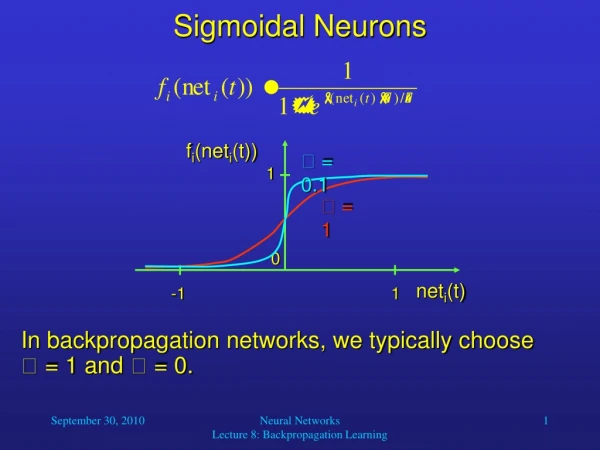
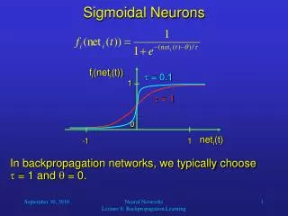
fi(neti(t)) = 0.1 1 = 1 0 neti(t) -1 1 Sigmoidal Neurons • In backpropagation networks, we typically choose = 1 and = 0. Neural Networks Lecture 8: Backpropagation Learning
Sigmoidal Neurons • This leads to a simplified form of the sigmoid function: We do not need a modifiable threshold , because we will use “dummy” inputs as we did for perceptrons. The choice = 1 works well in most situations and results in a very simple derivative of S(net). Neural Networks Lecture 8: Backpropagation Learning
Sigmoidal Neurons This result will be very useful when we develop the backpropagation algorithm. Neural Networks Lecture 8: Backpropagation Learning
Backpropagation Learning • Similar to the Adaline, the goal of the Backpropagation learning algorithm is to modify the network’s weights so that its output vector • op = (op,1, op,2, …, op,K) • is as close as possible to the desired output vector • dp = (dp,1, dp,2, …, dp,K) • for K output neurons and input patterns p = 1, …, P. • The set of input-output pairs (exemplars) {(xp, dp) | p = 1, …, P} constitutes the training set. Neural Networks Lecture 8: Backpropagation Learning
Backpropagation Learning • Also similar to the Adaline, we need a cumulative error function that is to be minimized: We can choose the mean square error (MSE) once again (but the 1/P factor does not matter): where Neural Networks Lecture 8: Backpropagation Learning
Terminology output vector o1 o2 • Example: Network function f: R3 R2 output layer hidden layer input layer x1 x2 x3 input vector Neural Networks Lecture 8: Backpropagation Learning
Backpropagation Learning • For input pattern p, the i-th input layer node holds xp,i. • Net input to j-th node in hidden layer: Output of j-th node in hidden layer: Net input to k-th node in output layer: Output of k-th node in output layer: Network error for p: Neural Networks Lecture 8: Backpropagation Learning
Backpropagation Learning • As E is a function of the network weights, we can use gradient descent to find those weights that result in minimal error. • For individual weights in the hidden and output layers, we should move against the error gradient (omitting index p): Output layer: Derivative easy to calculate Hidden layer: Derivative difficult to calculate Neural Networks Lecture 8: Backpropagation Learning
Backpropagation Learning • When computing the derivative with regard to wk,j(2,1), we can disregard any output units except ok: Remember that ok is obtained by applying the sigmoid function S to netk(2), which is computed by: Therefore, we need to apply the chain rule twice. Neural Networks Lecture 8: Backpropagation Learning
Backpropagation Learning We know that: Since We have: Which gives us: Neural Networks Lecture 8: Backpropagation Learning
Backpropagation Learning • For the derivative with regard to wj,i(1,0), notice that E depends on it through netj(1), which influences each ok with k = 1, …, K: Using the chain rule of derivatives again: Neural Networks Lecture 8: Backpropagation Learning
Backpropagation Learning • This gives us the following weight changes at the output layer: … and at the inner layer: Neural Networks Lecture 8: Backpropagation Learning
Backpropagation Learning Then we can simplify the generalized error terms: • As you surely remember from a few minutes ago: And: Neural Networks Lecture 8: Backpropagation Learning
Backpropagation Learning • The simplified error terms k and juse variables that are calculated in the feedforward phase of the network and can thus be calculated very efficiently. • Now let us state the final equations again and reintroduce the subscript p for the p-th pattern: Neural Networks Lecture 8: Backpropagation Learning
Backpropagation Learning • AlgorithmBackpropagation; • Start with randomly chosen weights; • while MSE is above desired threshold and computational bounds are not exceeded, do • for each input pattern xp, 1 p P, • Compute hidden node inputs; • Compute hidden node outputs; • Compute inputs to the output nodes; • Compute the network outputs; • Compute the error between output and desired output; • Modify the weights between hidden and output nodes; • Modify the weights between input and hidden nodes; • end-for • end-while. Neural Networks Lecture 8: Backpropagation Learning