Download
1 / 130
1.34k likes | 1.66k Vues
XI. Estimation of linear model parameters. XI.A Linear models for designed experiments XI.B Least squares estimation of the expectation parameters in simple linear models XI.C Generalized least squares (GLS) estimation of the expectation parameters in general linear models

E N D
XI. Estimation of linear model parameters XI.ALinear models for designed experiments XI.B Least squares estimation of the expectation parameters in simple linear models XI.C Generalized least squares (GLS) estimation of the expectation parameters in general linear models XI.D Maximum likelihood estimation of the expectation parameters XI.E Estimating the variance Statistical Modelling Chapter XI
where • y is an n1 vector of expected valuesfor the observations, • Y is an n1 vector of random variables for the observations, • X is an nq matrix with nq, • qis a q1 vector of unknown parameters, • V is an nn matrix, • is the variance component for the ith term in the variance model and • Si is the summation matrix for the ith term in the variance model. XI.A Linear models for designed experiments • In the analysis of experiments, the models that we have considered are all of the form • Note that generally the X matrices contain indicator variables, each indicating the observations that received a particular level of a (generalized) factor. Statistical Modelling Chapter XI
Summation matrices • Si is the matrix of 1s and 0s that forms the sums for the generalized factor corresponding to the ith term. • Now, • where • Mi is the mean operator for the ith term in the variance model, • n is the number of observational units and • fi is the number of levels of the generalized factor for this term. • For equally-replicated, generalized factors n/fi=gi where gi is the no. of repeats of each of its levels. • Consequently, the Ss could be replaced with Ms. Statistical Modelling Chapter XI
For example, variation model with Blocks random for RCBD with b= 3 and t= 4 Thus the model is of the form: Statistical Modelling Chapter XI
Classes of linear models • Firstly, linear models split into • expectation model is of full rank • expectation model is of less than full rank. • The rank of an expectation model is given by the following definitions — 2nd is equivalent to that given in chapter I. • Definition XI.1: The rank of an expectation model is equal to the rank of its X matrix. • Definition XI.2: The rank of an n q matrix X, with n q, is the number of linearly independent columns in X. • Such a matrix is of full rank when its rank equal q and is of less than full rank when its rank is less than q. • It will be less than full rank if the linear combination of some columns is equal to the same linear combination as some other columns. Statistical Modelling Chapter XI
Simple vs general models • Secondly, linear models split into those for which the variation model is • simple in that it is of the form s2In • more general form that involves more than one term. • For general linear models, S matrices in variation model can be written as direct products of I and J matrices. Definition XI.3: The direct-product operator is denoted and, if Ar and Bc are square matrices of order r and c, respectively, then Statistical Modelling Chapter XI
Expressions for S matrices in general models • When all the variation terms correspond to only unrandomized, and not randomized, generalized factors, use the following rule to derive these expressions. • Rule XI.1: The Si for the ith generalized factor from the unrandomized structure that involves s factors, is the direct product of s matrices, provided the s factors are arranged in standard order. • Taking the s factors in the sequence specified by the standard order, • for each factor in the ith generalized factor include an I matrix in the direct product and • J matrices for those that are not. • The order of a matrix in the direct product is equal to the number of levels of the corresponding factor. Statistical Modelling Chapter XI
Example IV.1 Penicillin yield (continued) • This experiment was an RCBD and its experimental structure is • Two possible models depending on whether Blends random or fixed. • For Blends fixed, • and taking the observations to be ordered in standard order for Blends then Flasks, • the only random term is BlendsFlasks and the maximal expectation and variation models are Statistical Modelling Chapter XI
Then the vectors and matrices in the maximal expectationmodel • are: Example IV.1 Penicillin yield (continued) • Suppose observations are • in standard order for Blend then Treatment; • with Flask renumbered within Blend to correspond to Treatment as in the prerandomization layout. • Analysis for prerandomization and randomized layouts must be same as prerandomization layout is one of the possible randomized arrangements. • Can write the Xs as direct products: • XB=I5 14 • XT=15 I4 Statistical Modelling Chapter XI
Example IV.1 Penicillin yield (continued) • Clearly, sum of indicator variables (columns) in XB and sum of those in XT both equal 120 • So the expectation model involving the X matrix [XBXT] is of less than full rank — its rank is b + t-1. • The linear model is a simple linear model because the variance matrix is of the form s2In. • That is, the observations are assumed to have the same variance and to be uncorrelated. Statistical Modelling Chapter XI
Example IV.1 Penicillin yield (continued) • On the other hand, for Blends random, • the random terms are Blends and BlendsFlasks and • the maximal expectation and variation models are • In this case the expectation is of full rank as XT consists of t linearly independent columns. • However, it is a general, not a simple, linear model as the variance matrix is not of the form s2In. Statistical Modelling Chapter XI
Clearly, occurs down the diagonal and occurs in diagonal 44 blocks. Example IV.1 Penicillin yield (continued) • The form is illustrated for b = 3, t = 4 below, the extension to b = 5 being obvious. • Model allows for covariance, and hence correlation, between flasks from the same blend. Statistical Modelling Chapter XI
Hence, the direct product for is I5 I4 and it involves two I matrices because both unrandomized factors, Blends and Flasks, occur in BlendsFlasks. • The direct product for is I5 J4 and it involves an I and a J because the factor Blends is in this term but Flasks is not. Example IV.1 Penicillin yield (continued) • The direct-product expressions for both Vs conform to rule XI.1. • Recall, the units are indexed with Blocks then Flasks. Statistical Modelling Chapter XI
Example IX.1 Production rate experiment (revisited) • Layout: • The experimental structure for this experiment was: Statistical Modelling Chapter XI
Example IX.1 Production rate experiment (revisited) • Suppose all the unrandomized factors are random • So the maximal expectation and variation models are, symbolically • y=E[Y] = MethodsSources • var[Y] = Factories + FactoriesAreas + FactoriesAreasParts. • That is Statistical Modelling Chapter XI
In this matrix • will occur down the diagonal, • will occur in 3 3 blocks down the diagonal and • will occur in 9 9 blocks down the diagonal. Example IX.1 Production rate experiment (revisited) • Now if the observations are arranged in standard order with respect to the factors Factories, Areas and then Parts, we can use rule XI.1 to obtain the following direct-product expression for V. • So this model allows for • covariance between parts from the same area and • a different covariance between areas from the same factory. Statistical Modelling Chapter XI
Example IX.1 Production rate experiment (revisited) • Actually, in ch. IX, Factories was assumed fixed and so • So the rules still apply as terms in V only involve unrandomized factors • This model only allows for • covariance between parts from the same area. Statistical Modelling Chapter XI
XI.B Least squares estimation of the expectation parameters in simple linear models • Want to estimate the parameters q in the expectation model by establishing their estimators. • There are several different methods for doing this. • A common method is the method of least squares, as in the following definition originally given in chapter I. Statistical Modelling Chapter XI
a) Ordinary least squares estimators for full-rank expectation models • Definition XI.4: Let Y=Xq + e where • X is an nq matrix of rank mq with nq, • qis a q1 vector of unknown parameters, • e is an n1 vector of errors with mean 0 and variance s2In. The least ordinary least squares (OLS) estimator of q is the value of q that minimizes • Note applies to the less-than-full rank case Statistical Modelling Chapter XI
Least squares estimators of q • Theorem XI.1: Let Y=Xq + e where • Y is an n1 vector of random variables for the observations, • X is an nq matrix of full rank with nq, • qis a q1 vector of unknown parameters, • e is an n1 vector of errors with mean 0 and variance s2In. The ordinary least squares estimator of q is given by • (The ‘^’ denotes estimator) • Proof: Need to set differential of e'e= (Y – Xq)'(Y – Xq) to zero (see notes for details); • Yields the normal equations whose solution is given above. Statistical Modelling Chapter XI
Estimator of y • Using definition I.7 (expected values), an estimator of the expected values is • Now for experiments • the X matrix consists of indicator variables and • the maximal expectation model is generally the sum of terms each of which is an X matrix for a (generalized) factor and an associated parameter vector. • In cases where maximal expectation model involves a single term corresponding to just one generalized factor, • the model is necessarily of full rank and • the OLS estimator of its parameters is particularly simple. Statistical Modelling Chapter XI
Example VII.4 22 Factorial experiment • To aid in proofs coming up consider a two-factor factorial experiment (as in chapter 7, Factorial experiments). • Suppose there are the two factors A and B with a=b= 2, r= 3 and n= 12. • Assume that data is ordered for A then B then replicates. • The maximal model involves a single term corresponding to the generalized factor AB — it is That is, each column of XAB indicates which observations received one of the combinations of the levels of A and B. Statistical Modelling Chapter XI
So we require Example VII.4 22 Factorial experiment (continued) • Now, from theorem XI.1 (OLS estimator), the estimator of the expectation parameters is given by Statistical Modelling Chapter XI
Example VII.4 22 Factorial experiment (continued) — obtaining inverse • Notice in the above that • rows of XAB are columns of XAB • each element in product is of the form • where xi and xj are the n-vectors for the ith and jth columns of X, respectively. • i.e. sum of pairwise products of elements of ith and jth columns of X. Statistical Modelling Chapter XI
Example VII.4 22 Factorial experiment (continued) — obtaining product • where Yij. is the sum over the replicates for the ijth combination of A and B. Statistical Modelling Chapter XI
Example VII.4 22 Factorial experiment (continued) — obtaining parameter estimates • where is the mean over the replicates for the ijth combination of A and B. Statistical Modelling Chapter XI
Example VII.4 22 Factorial experiment (continued) — obtaining estimator of expected values • where is the mean operator producing the n-vector of means for the combinations of A and B. Statistical Modelling Chapter XI
Proofs for expected values for a single-term model • First prove that model is of full rank and then derive the OLS estimator. • Lemma XI.1: Let X be an n f matrix with n≥ f. Then rank(X) =rank(XX). Proof: not given. Statistical Modelling Chapter XI
Proofs for expected values for a single-term model (continued) • Lemma XI.2: Let Y=Xq + e where X is an n f matrix corresponding to a generalized factor, F say, with f levels and n≥ f. Then, the rank of X is f so that X is of full rank. • Proof: Lemma XI.1 states that rank(X) =rank(XX) and it is easier to derive the rank of XX. • To do this we need to establish a general expression for XX which we do by considering the form of X. Statistical Modelling Chapter XI
Proofs for expected values for a single-term model (continued) • Now • n rows of X correspond to observational units in the experiment and • f columns to the levels of the generalized factor. • All the elements of X are either 0 or 1 • In the ith column, a 1 occurs for those units with the ith level of the generalized factor so that, if the ith level of the generalized factor is replicated gi times, there will be gi 1s in the ith column. • In each row of X there will be a single 1 as only one level of the generalized factor can be observed with each unit if it is the ith level of the generalized factor that occurs on the unit, then the 1 will occur in the ith column of X. Statistical Modelling Chapter XI
Proofs for expected values for a single-term model (continued) • Considering the f f matrix XX • its ijth element is the product of the ith column, as a row vector, with the jth column as given in the following expression (see example above): • When i=j, the 2 columns are same and the products are either of two 1s or two 0s, so • product is 1 for units that have ith level of generalized factor and • sum will be gi. • When i≠j, have product of vector for ith column, as a row vector, with that for jth column. • As each unit can receive only one level for the generalized factor, it cannot receive both ith and jth levels and the products are either two 0s or a 1 and a 0. • Consequently, sum is zero. Statistical Modelling Chapter XI
Proofs for expected values for a single-term model (continued) • It is concluded that XX is a f f diagonal matrix with diagonal elements gi. • Hence, in this case, the rank(X) =rank(XX) =f and so X is of full rank. Statistical Modelling Chapter XI
The ordinary least squares estimator of q is denoted by and is given by double over-dots indicate not n-vector, but f-vector. where is the f-vector of means for the levels of the generalized factor F. Proofs for expected values for a single-term model (continued) • Theorem XI.2: Let Y=Xq + e where • X is an n f matrix corresponding to a generalized factor, F say, with f levels and n≥ f. • qis a f 1 vector of unknown parameters, • e is an n1 vector of errors with mean 0 and variance s2In. Statistical Modelling Chapter XI
Proof: From theorem XI.1(OLS estimator) we have that the OLS estimator is • Consequently, (XX)-1 is a diagonal matrix with diagonal elements Proofs for expected values for a single-term model (continued) • Need expressions for XX and XY in this special case . • In the proof of lemma XI.2 it was shown that XX is a f f diagonal matrix with diagonal elements gi. Statistical Modelling Chapter XI
Proofs for expected values for a single-term model (continued) • Now XY is an f-vector whose ith element is the total for the ith level of the generalized factor of the elements of Y. • This can be seen when it is realized that the ith element of XY is the product of the ith column of X with Y. • Clearly, the result will be the sum of the elements of Y corresponding to elements of the ith column of X that are one: • those units with the ith level of the generalized factor. • Finally, taking the product of (XX)-1 with XY divides each total by its replication forming the f-vector of means as stated. Statistical Modelling Chapter XI
Proofs for expected values for a single-term model (continued) • Corollary XI.1: With the model for Y as in theorem XI.2, the estimator of the expected values are given by • where • is the n-vector an element of which is the mean for the level of the generalized factor F for the corresponding unit and • MF is the mean operator that replaces each observation in Y with the mean for the corresponding level of the generalized factor F. Statistical Modelling Chapter XI
Proof: Now and, as stated in proof of lemma XI.2 (rank X), each row of X contains a single 1 • if it is the ith level of the generalized factor that occurs on the unit, then the 1 will occur in the ith column of X. • So corresponding element of will be the ith element of which is the mean for the ith level of the generalized factor F and • To show that , we have from theorem XI.1 (OLS estimator) that • Letting yields • Now, given also, MF must be the mean operator that replaces each observation in Y with the mean for the corresponding level of the F. Proofs for expected values for a single-term model (continued) Statistical Modelling Chapter XI
Example XI.1 Rat experiment • See lecture notes for this example that involves a single, original factor whose levels are unequally replicated. Statistical Modelling Chapter XI
b) Ordinary least squares estimators for less-than-full-rank expectation models • The model for the expectation is still of the form E[Y]=Xq but in this case the rank of X is less than the number of columns. • Now rank(X) =rank(XX) =m < q and so there is no inverse of XX to use in solving the normal equations • Our aim is to show that, in spite of this and the difficulties that ensue, the estimators are functions of means. • For example, the maximal, less-than-full-rank, expectation model for an RCBD is: • yB+T=E[Y] =XBb + XTt • Will show, with some effort, the estimator of the expected values is: Statistical Modelling Chapter XI
In the full rank model XX is nonsingular and so (XX)-1 exists and the normal equations have the one solution: • In a less-than-full-rank model there are infinitely many solutions to the normal equations. Less-than-full-rank vs full-rank model • In the full rank model it is assumed that the parameters specified in the model are unique. There exists exactly one set of real numbers {q1, q2, …, qq} that describes the system. In the less-than-full-rank model there are infinitely many sets of real numbers that describe the system. For our example, there are infinitely many choices for {b1, …, bb, t1, …, tt}. The model parameters are said to be nonidentifiable. • In the full rank model all linear functions of {q1, q2, …, qq} can be estimated unbiasedly. • In the less-than-full-rank model some functions can while others cannot. Want to identify functions with invariant estimated values. Statistical Modelling Chapter XI
Example XI.2 The RCBD • Simplest model that is less than full rank is the maximal expectation model for the RCBD, E[Y] = Blocks + Treats. • Generally, RCBD involves b blocks with t treatments so that there are n=bt observations. • The maximal model used for an RCBD, in matrix terms, is: yB+T=E[Y] =XBb + XTt and var[Y] =s2In • However, as previously mentioned, the model is not of full rank because the sums of the columns of both XB and XT are equal to 1n. • Consequently, for X= [XBXT], rank(X) =rank(XX) =b + t- 1 Statistical Modelling Chapter XI
Illustration for b=t=2 that the parameters are nonidentifiable • Suppose following information is known about the parameters: • Then the parameters are not identifiable for: • if b1= 5, then t1= 5, t2= 10 and b2= 7; • if b1= 6, then t1= 4, t2= 9 and b2= 8. • Clearly can pick a value for any one of the parameters and then find values of the others that satisfy the above equations. • Infinitely many possible values for the parameters. • However, no matter what values are taken for b1, b2, t1 and t2, the value of b2-b1= 2 and of t2 - t1= 5; • these functions are invariant. Statistical Modelling Chapter XI
Coping with less-than-full-rank models • Extend estimation theory presented in section a), Ordinary least squares estimators for full-rank expectation models. • Involves obtaining solutions to the normal equations using generalized inverses. Statistical Modelling Chapter XI
Introduction to generalized inverses • Suppose that we have a system of n linear equations in q unknowns such as Ax=y • where • A is an nq matrix of real numbers, • x is a q-vector of unknowns and • y is a n-vector of real numbers. • There are 3 possibilities: • the system is inconsistent and has no solution; • the system is consistent and has exactly one solution; • the system is consistent and has many solutions. Statistical Modelling Chapter XI
Theorem XI.3: Let E[Y]=Xq be a linear model for the expectation. Then the system of normal equations • is consistent. • Proof: not given. Consistent vs inconsistent equations • Consider the following equations: x1 + 2x2= 7 3x1 + 6x2= 21 • They are consistent in that the solution of one will also satisfy the second because the second equation is just 3 times the first. • However, the following equations are inconsistent in that it is impossible to satisfy both at the same time: x1 + 2x2= 7 3x1 + 6x2= 24 • Generally, to be consistent, any linear relations on the left of the equations must also be satisfied by the righthand side of the equation. Statistical Modelling Chapter XI
Generalized inverses • Definition XI.5: Let A be an nq matrix. A qn matrix A- such that AA-A = A is called a generalised inverse (g-inverse for short) for A. • Any matrix A has a generalized inverse but it is not unique unless A is nonsingular, in which case A-=A-1. Statistical Modelling Chapter XI
Example XI.3 Generalized inverse of a 22 matrix It is easy to see that the following matrices are also generalized inverse for A: This illustrates that generalized inverses are not necessarily unique. Statistical Modelling Chapter XI
An algorithm for finding generalized inverses To find a generalized inverse A- for an matrix A of rank m: • Find any mm minor H of A i.e. the matrix obtained by selecting any m rows and any m columns of A. • Find H-1. • Replace H in A with (H-1)'. • Replace all other entries in A with zeros. • Transpose the resulting matrix. Statistical Modelling Chapter XI
Properties of generalized inverses • Let A be an nq matrix of rank m with n q m. • Then • A-A and AA- are idempotent. • rank(A-A) =rank(AA-) =m. • If A- is a generalized inverse of A, then (A-)' is a generalized inverse of A'; that is, (A-)' = (A')-. • (A'A)-A' is a generalized inverse of A so that A=A(A'A)-(A'A) and A'= (A'A)(A'A)-A'. • A(A'A)-A' is unique, symmetric and idempotent as it is invariant to the choice of a generalized inverse. Furthermore rank(A(A'A)-A') =m. Statistical Modelling Chapter XI
Generalized inverses and the normal equations • Lemma XI.3: Let Ax=y be consistent. Then x=A-y is a solution to the system where A- is any generalized inverse for A. • Proof: not given. Statistical Modelling Chapter XI