Download
1 / 74
750 likes | 1.07k Vues
Stochastic Population Forecasting and ARIMA time series modelling Lectures QMSS Summer School, 2 July 2009. Nico Keilman Department of Economics, University of Oslo . Stochastic. Stochastic (from the Greek "Στόχος" for "aim" or "guess") means random.

E N D
Stochastic Population ForecastingandARIMA time series modellingLectures QMSS Summer School, 2 July 2009 Nico Keilman Department of Economics, University of Oslo
Stochastic • Stochastic (from the Greek "Στόχος" for "aim" or "guess") means random. • A stochastic process is one whose behaviour is non-deterministic in that a system's subsequent state is determined both by the process's predictable actions and by a random element. • In a stochastic population forecast, uncertainty is made explicit: random variables are part of the forecast model.
Stochastic population forecast Future population / births / deaths /migrations as probability distributions, not one number (perhaps three)
Why Stochastic Population Forecasts (SPF)? Users should be informed about the expected accuracy of the forecast - probability of alternative future paths? - which forecast horizon is reasonable? Traditional deterministic forecast variants (e.g. High, Medium, Low) - do not quantify uncertainty Prob(MediumPop) = 0 !! - give a misleading impression of uncertainty (example later) - leave room for politically motivated choices by the user
Outline • Uncertainty of population forecasts • Principles of SPF • Time series models (selected examples) • Alho’s scaled model for error • Examples from UPE • Using a SPF Focus on national forecasts
How uncertain are population forecasts? Empirical findings – historical forecasts evaluated against actual population numbers (ex post facto)
Main findings for official forecasts in Western countries • Uncertainty in forecasts of certain population variables surprisingly large • Forecasts for the young and the old age groups are the least reliable • Forecast errors increase as forecast interval lengthens • Large uncertainty for small countries • Large uncertainty for countries that are strongly affected by migration • European forecasts have not become more accurate since WW2
Why uncertain? • Data quality (LDC’s) • Social science predictions, no accurate behavioural theory • Rely on observed regularities instead Problems when sudden trend shifts occur - stagnation life expectancy men 1950s - baby boom/baby bust
Traditional population forecasts do not give a correct impression of uncertainty
Example: Old Age Dependency Ratio (OADR) for Norway in 2060Source: Statistics Norway population forecast of 2005 High Middle Low |H-L|/M millions (%) POP67+ 1.55 1.33 1.13 31 POP20-66 4.03 3.39 2.83 36 OADR 0.38 0.39 0.40 4
Two major problems • Wide margins for some variables, narrow margins for others • Narrow margins in the short run,wide margins in the long run - implicitly assumed perfect autocorrelation (and sometimes perfect correlation across components)
Coverage probabilities for H-L margin of total population in official forecasts 2010 2050 Statistics Norway 47% 78% Statistics Sweden • Fertility 19% 32% • Mortality 4% 20% • Migration 1% 34% Sources: Stochastic population forecasts from UPE Traditional forecasts from Statistics Norway and Statistics Sweden
Cohort-component method Deterministic population forecast Needed for the country in question: annual assumptions on future • Fertility Total Fertility Rate • Mortality Life expectancy at birth M/F • Migration Net immigration • as well as rates (fertility, mortality) & numbers (migration) by age & sex
Stochastic Population Forecast: How? • Cohort-component method • Random rates for fertility and mortality, random numbers for net-migration • Normal distributions in the log scale (rates) or in the original scale (migration numbers) - expected values (“point predictions”) – cf. Medium variant in traditional deterministic forecast - standard deviations - correlations (age, time, sex, components, countries)
SPF: How? (cntnd) • Joint distribution of all random input variables (rates, migration numbers) • In practice: simplifications, e.g. - independence of components (fertility, mortality, migration) - correlation between male and female mortality (constant across ages, time) • One random draw from all prob. distributions one sample path • Repeated draws thousands of sample paths
SPF: How? (cntnd) Three main approaches: uncertainty parameters based on historical errors expert knowledge statistical model
SPF: Examples Multivariate time series models for all parameters of interest Examples for Norway 1995-2050, see http://folk.uio.no/keilman/6-15.pdf and European countries 2003-2050, see http://www.stat.fi/tup/euupe/index_en.html Alho’s scaled model for error, implemented in PEP (Program for Error Propagation) Example for aggregate of 18 European countries 2003-2050, see http://www.stat.fi/tup/euupe/index_en.html
Time series example, Norway:log(TFR) = ARIMA(1,1,0) Zt = 0.67Zt-1 + εt-1 , Zt = log(TFRt) - log(TFRt-1) (0.10)
Prediction intervals, age-specific fertility rates, Norway 2050
Time series models for • parameters of Gamma model for age-specific fertility (TFR, MAC, variance in age at childbearing) • e0 • parameters of Heligman-Pollard model for age-specific mortality • immigration numbers • emigration numbers (deterministic age patterns for both migration flows) 5000 simulations
Time series models, two examples 1. Autoregressive model of order 1 - AR(1) Zt = φZt-1 + εt |φ| < 1, εt i.i.d random variables, zero expectation, constant variance – ”white noise” Var(Zt) = Var(εt)(1- φ2t)/(1- φ2) constant (in the long run – large t) For large t: k-step ahead autocorrelation Corr(Zt, Zt+k) equals φk , independent of time
2. Random Walk - RW Zt = Zt-1 + εt Var(Zt) = t*Var(εt) unbounded for large t Independent increments (zero autocorrelation)
Forecasts and 95% prediction intervals for net migration. Data 1960-2000 Outliers: 1989 AR(1) & const:Zt=5688+0.76Zt-1+εtOutliers: 1962, 1988AR(1) & const:Zt=7819+0.39Zt-1+εt
Forecasts and 67%, 80%, and 95% prediction intervals for the TFR. Data 1950-2000. Observed TFR-value for the year 2000 is given as “y2000” Model: AR(1) & constant Zt (=logTFRt) = 0.001 + 0.988Zt-1 + εt
Forecasts and 67%, 80%, and 95% prediction intervals for the TFR. Data 1900-2000. Observed TFR-value for the year 2000 is given as “y2000” Model: AR(1) & constant Outliers 1920, 1942Zt (=logTFRt) = -0.003 + 0.995Zt-1 + εt
Forecasts and 67%, 80%, and 95% prediction intervals for the TFR. Data 1950-2000. Observed TFR-value for the year 2000 is given as “y2000” Model: AR(2) & constant Zt (=logTFRt) = 0.002 + 0.941Zt-1 - 0.408Zt-2 + εt
Forecasts and 67%, 80%, and 95% prediction intervals for the TFR. Data 1900-2000. Observed TFR-value for the year 2000 is given as “y2000” Model: AR(2)-ARCH(1) Outliers 1919, 1920, 1940, 1941Zt (=logTFRt) = 0.005 + 0.981Zt-1 + vt + dummiesvt = 0.214 vt-2 + εt,εt = (√ht)et, ht = 7E-4+0.708(εt2)
Time series approach to SPF + conceptually simple - inflexible Alternative: Alho’s scaled model for error Implemented in Program for Error Propagation (PEP) http://www.joensuu.fi/statistics/software/pep/pepstart.htm .
Scaled model for error Suppose the true age-specific rate in age j during forecast year t > 0 is of the form R(j,t) = F(j,t)exp(X(j,t)), where F(j,t) is the point forecast, and X(j,t) is the relative error
Suppose that the error processes are of the form X(j,t) = ε(j,1) + ... + ε(j,t) with error increments of the form ε(j,t) = S(j,t)(ηj + δ(j,t)) S(j,t) deterministic scales. δ(j,t) are independent over time t. δ(j,t) are independent of ηj for all t and j ηj ~ N(0, κ), δ(j,t) ~ N(0, 1 - κ) , 0 ≤ κ ≤ 1 Note that Var(ε(j,t)) = S(j,t)2 A positive kappa means that there is systematic error in the time trend of the rate.
κ = Corr[ε(j,t), ε(j,t+h)] for all h > 0, thus κ is the (constant) autocorrelation between the error increments. Together, the autocorrelation κ and the scale S(j,t) determine the variance of the relative error X(j,t). Ex. 1. Under a random walk model the error increments are uncorrelated with κ = 0. Ex. 2. The model with constant scales (S(j,t)=S(j)) can be interpreted as a random walk with a random drift. The relative importance of the two components is determined by κ.
Migration Migration (net) is represented in absolute terms Dependence on age is deterministic, given by a fixed distribution g(j,x) over age x The error of net migration in age x, for sex j, during year t > 0, is additive and of the form Y(j,x,t) = S(j,t)g(j,x)(ηj + δ(j,t))
Key properties of the scaled model • The choice of the scales S(j,t) is unrestricted. Hence any sequence of non-decreasing error variances can be matched (e.g. heteroscedasticity) • Any sequence of cross-correlations over ages can be majorized using the AR(1) models of correlation • Any sequence of autocorrelations for the error increments can be majorized.
Scaled model for error Used for UPE project: Uncertain Population of Europe • 18 countries: EU15 + Iceland, Norway, Switzerland (EEA+) • 2003 – 2050 • Probability distributions specified on the basis of - time series analysis (TFR, e0, net-migr.) - empirical forecast errors - expert judgement • 3000 simulations for each country, PEP • http://www.stat.fi/tup/euupe/index_en.html
Population size EEA+median (black), 80% prediction intervals (red) 77% chance > 400 million in 2050 (UN)83% chance > 392 million in 2050 (2003)