Probability Theory General Probability Rules
Probability Theory General Probability Rules PBS Chapter 5.1 © 2009 W.H. Freeman and Company Objectives (PBS Chapter 5.1) General probability rules Independence and the multiplication rule Applying the multiplication rule The general addition rule Probability Rules (review)

Probability Theory General Probability Rules
E N D
Presentation Transcript
Probability TheoryGeneral Probability Rules PBS Chapter 5.1 © 2009 W.H. Freeman and Company
Objectives (PBS Chapter 5.1) General probability rules • Independence and the multiplication rule • Applying the multiplication rule • The general addition rule
Probability Rules (review) We already met the following four rules in Chapter 4: 1) Probabilities range from 0 (no chance of the event) to1 (the event has to happen). For any event A, 0 ≤P(A) ≤ 1 Probability of getting a Head = 0.5 We write this as: P(Head) = 0.5 P(neither Head nor Tail) = 0 P(getting either a Head or a Tail) = 1 2) Because some outcome must occur on every trial, the sum of the probabilities for all possible outcomes (the sample space) must be exactly 1. P(sample space) = 1 Coin toss: S = {Head, Tail} P(head) + P(tail) = 0.5 + 0.5 =1 P(sample space) = 1
Coin Toss Example: S ={Head, Tail} Probability of heads = 0.5 Probability of tails = 0.5 Probability rules (contd) 3) The complement of any event A is the event that A does not occur, written as Ac. The complement rule states that the probability of an event not occurring is 1 minus the probability that is does occur. P(not A) = P(Ac) = 1 −P(A) Tailc = not Tail = Head P(Tailc) = 1 −P(Head) = 0.5 Venn diagram: Sample space made up of an event A and its complementary Ac, i.e., everything that is not A.
Venn diagrams: A and B disjoint Probability rules (contd ) 4) Two events A and B are disjoint if they have no outcomes in common and can never happen together. The probability that A or B occurs is then the sum of their individual probabilities. P(A or B) = “P(A U B)” = P(A) + P(B) This is the addition rule for disjoint events. A and B not disjoint Example:If you flip two coins, and the first flip does not affect the second flip: S = {HH, HT, TH, TT}. The probability of each of these events is 1/4, or 0.25. The probability that you obtain “only heads or only tails” is:P(HH or TT) = P(HH) + P(TT) = 0.25 + 0.25 = 0.50
Independence Two events are independent if the probability that one event occurs on any given trial of an experiment is not affected or changed by the occurrence of the other event. When are trials not independent? Imagine that these coins were spread out so that half were heads up and half were tails up. Close your eyes and pick one. The probability of it being heads is 0.5. However, if you don’t put it back in the pile, the probability of picking up another coin and having it be heads is now less than 0.5. The trials are independent only when you put the coin back each time. It is called sampling with replacement.
Multiplication Rule for Independent Events Two events A and B are independent if knowing that one occurs does not change the probability that the other occurs. If A and B are independent, P(A and B) = P(A)P(B) This is the multiplication rule for independent events. Two consecutive coin tosses: P(first Tail and second Tail) = P(first Tail) * P(second Tail) = 0.5 * 0.5 = 0.25 Venn diagram: Event A and event B. The intersection represents the event {A and B} and outcomes common to both A and B.
Independent vs. Disjoint Events • Disjoint events are not independent. • If A and B are disjoint, then the fact that A occurs tells us that B cannot occur. So A and B are not independent. • Independence cannot be pictured in a Venn Diagram.
Applying the Multiplication Rule • If two events A and B are independent, the event that A does not occur is also independent of B. • The Multiplication Rule extends to collections of more than two events, provided that all are independent. • Example: A transatlantic data cable contains repeaters to amplify the signal. Each repeater has probability 0.999 of functioning without failure for 25 years. Repeaters fail independently of each other. Let A1 denote the event that the first repeater operates without failure for 25 years, A2 denote the event that the second repeater operates without failure for 25 years, and so on. The last transatlantic cable had 662 repeaters. The probability that all 662 will work for 25 years is: P(A1 and A2 and…and A662) = 0.999662 = 0.516
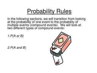
General addition rule General addition rule for any two events A and B: The probability that A occurs, or B occurs, or both events occur is: P(A or B) = P(A) + P(B) – P(A and B) What is the probability of randomly drawing either an ace or a heart from a deck of 52 playing cards? There are 4 aces in the pack and 13 hearts. However, 1 card is both an ace and a heart. Thus: P(ace or heart) = P(ace) + P(heart) – P(ace and heart) = 4/52 + 13/52 - 1/52 = 16/52 ≈ .3
Probability TheoryThe Binomial and Poisson Distributions PBS Chapters 5.2 and 5.3 © 2009 W. H. Freeman and Company
Objectives (PBS Chapter 5.2 and 5.3) Binomial and Poisson Distributions • The binomial setting • Binomial Probabilities • Binomial mean and standard deviation • The Normal approximation • The Poisson setting • The Poisson model
Binomial Setting Binomial distributions are models for some categorical variables, typically representing the number of successes in a series of n trials. The observations must meet these requirements: • The total number of observations n is fixed in advance. • The outcomes of all n observations are statistically independent. • Each observation falls into just one of 2 categories: success and failure. • All n observations have the same probability of “success,” p. We record the next 50 births at a local hospital. Each newborn is either a boy or a girl; each baby is either born on a Sunday or not.
Binomial Distribution The distribution of the count X of successes in the binomial setting is the binomial distribution with parameters n and p:B(n,p). • The parameter n is the total number of observations. • The parameter p is the probability of success on each observation. • The count of successes X can be any whole number between 0 and n. A coin is flipped 10 times. Each outcome is either a head or a tail. The variable X is the number of heads among those 10 flips, our count of “successes.” On each flip, the probability of success, “head,” is 0.5. The number X of heads among 10 flips has the binomial distribution B(n = 10, p = 0.5).
Applications for binomial distributions Binomial distributions describe the possible number of times that a particular event will occur in a sequence of observations. They are used when we want to know about the occurrence of an event, not its magnitude. • In a clinical trial, a patient’s condition may improve or not. We study the number of patients who improved, not how much better they feel. • Is a person ambitious or not? The binomial distribution describes the number of ambitious persons, not how ambitious they are. • In quality control we assess the number of defective items in a lot of goods, irrespective of the type of defect.
Binomial Probabilities The number of ways of arranging k successes in a series of n observations (with constant probability p of success) is the number of possible combinations (unordered sequences). This can be calculated with the binomial coefficient: Where k = 0, 1, 2, ..., or n.
Binomial formulas • The binomial coefficient “n_choose_k” uses the factorialnotation “!”. • The factorial n! for any strictly positive whole number n is: n! = n × (n − 1) × (n − 2) × · · · × 3 × 2 × 1 • For example: 5! = 5 × 4 × 3 × 2 × 1 = 120 • Note that 0! = 1.
Calculations for binomial probabilities The binomial coefficient counts the number of ways in which k successes can be arranged among n observations. The binomial probability P(X = k) is this count multiplied by the probability of any specific arrangement of the k successes: The probability that a binomial random variable takes any range of values is the sum of each probability for getting exactly that many successes in n observations. P(X≤ 2) = P(X = 0) + P(X = 1) + P(X = 2)
Finding binomial probabilities: tables • You can also look up the probabilities for some values of n and p in Table C in the back of the book. • The entries in the table are the probabilities P(X = k) of individual outcomes. • The values of p that appear in Table C are all 0.5 or smaller. When the probability of a success is greater than 0.5, restate the problem in terms of the number of failures.
Color blindness The frequency of color blindness (dyschromatopsia) in the Caucasian American male population is estimated to be about 8%. We take a random sample of size 25 from this population. What is the probability that exactly five individuals in the sample are color blind? • Use Excel’s “=BINOMDIST(number_s,trials,probability_s,cumulative)” P(x= 5) = BINOMDIST(5, 25, 0.08, 0) = 0.03285 • P(x= 5) = (n! / k!(n k)!)pk(1 p)n-k = (25! / 5!(20)!) 0.0850.925P(x= 5) = (21*22*23*24*24*25 / 1*2*3*4*5) 0.0850.9220P(x= 5) = 53,130 * 0.0000033 * 0.1887 = 0.03285
Binomial mean and standard deviation The center and spread of the binomial distribution for a count X are defined by the mean m and standard deviation s: a) b) Effect of changing p when n is fixed. a) n = 10, p = 0.25 b) n = 10, p = 0.5 c) n = 10, p = 0.75 For small samples, binomial distributions are skewed when p is different from 0.5. c)
Normal approximation If n is large, and p is not too close to 0 or 1, the binomial distribution can be approximated by the normal distribution N(m = np,s2 = np(1 p)) Practically, the Normal approximation can be used when both np≥10 and n(1 p) ≥10. If X is the count of successes in the sample the sampling distributions for large n, is: • X approximately N(µ = np,σ2 = np(1 − p))
The Poisson Setting • A count X of successes has a Poisson distribution in the Poisson setting: • The number of successes that occur in any unit of measure is independent of the number of successes that occur in any non-overlapping unit of measure. • The probability that a success will occur in a unit of measure is the same for all units of equal size and is proportional to the size of the unit. • The probability that 2 or more successes will occur in a unit approaches 0 as the size of the unit becomes smaller.
Poisson Distribution • The distribution of the count X of successes in the Poisson setting is the Poisson distribution with meanμ. The parameter μis the mean number of successes per unit of measure. • The possible values of X are the whole numbers 0, 1, 2, 3, ….If k is any whole number 0 or greater, then P(X = k) = (e-μμk)/k! • The standard deviation of the distribution is the square root of μ.
Probability TheoryConditional Probability PBS Chapter 5.4 © 2009 W.H. Freeman and Company
Objectives (PBS Chapter 5.4) Conditional Probability • General multiplication rule • Conditional probability and independence • Tree diagrams • Bayes’s rule
General Multiplication Rule • Conditional probability gives the probability of one event under the condition that we know another event. • General multiplication rule: The probability that any two events, A and B, happen together is: P(A and B) = P(A)P(B|A) Here P(B|A) is the conditional probability that B occurs, given the information that A occurs.
Conditional probability Conditional probabilities reflect how the probability of an event can change if we know that some other event has occurred/is occurring. • Example: The probability that a cloudy day will result in rain is different if you live in Los Angeles than if you live in Seattle. • Our brains effortlessly calculate conditional probabilities, updating our “degree of belief” with each new piece of evidence. The conditional probability of event B given event A is:(provided that P(A) ≠ 0)
Independent Events Recall: A and B are independent when they have no influence on each other’s occurrence. • Two events A and B that both have positive probability are independent if P(B|A) = P(B) • The general multiplication rule then becomes: P(A and B) = P(A)P(B) • What is the probability of randomly drawing an ace of hearts from a deck of 52 playing cards? There are 4 aces in the pack and 13 hearts. • P(heart|ace) = 1/4 P(ace) = 4/52 • P(ace and heart) = P(ace)* P(heart|ace) = (4/52)*(1/4) = 1/52 Notice that heart and ace are independent events.
Tree diagram for chat room habits for three adult age groups 0.47 Internet user Tree diagrams Conditional probabilities can get complex, and it is often a good strategy to build a probability tree that represents all possible outcomes graphically and assigns conditional probabilities to subsets of events. P(chatting) = 0.136 + 0.099 + 0.017 = 0.252 About 25% of all adult Internet users visit chat rooms.
Diagnosis sensitivity 0.8 Disease incidence Positive Cancer 0.0004 False negative Negative 0.2 Mammography 0.1 False positive Positive 0.9996 No cancer Negative Incidence of breast cancer among women ages 20–30 0.9 Diagnosis specificity Mammography performance Breast cancer screening If a woman in her 20s gets screened for breast cancer and receives a positive test result, what is the probability that she does have breast cancer? She could either have a positive test and have breast cancer or have a positive test but not have cancer (false positive).
Diagnosis sensitivity Disease incidence Positive Cancer False negative Negative Mammography False positive Positive No cancer Negative Diagnosis specificity 0.8 0.0004 0.2 0.1 0.9996 Incidence of breast cancer among women ages 20–30 0.9 Mammography performance Possible outcomes given the positive diagnosis: positive test and breast cancer or positive test but no cancer (false positive). This value is called the positive predictive value, or PV+. It is an important piece of information but, unfortunately, is rarely communicated to patients.
Bayes’s rule An important application of conditional probabilities is Bayes’s rule. It is the foundation of many modern statistical applications beyond the scope of this textbook. * If a sample space is decomposed in k disjoint events, A1, A2, … , Ak— none with a null probability but P(A1) + P(A2) + … + P(Ak) = 1, * And if C is any other event such that P(C) is not 0 or 1, then: However, it is often intuitively much easier to work out answers with a probability tree than with these lengthy formulas.
Diagnosis sensitivity Disease incidence Positive Cancer False negative Negative Mammography False positive Positive No cancer Negative Diagnosis specificity If a woman in her 20s gets screened for breast cancer and receives a positive test result, what is the probability that she does have breast cancer? 0.8 0.0004 0.2 0.1 0.9996 Incidence of breast cancer among women ages 20–30 0.9 Mammography performance This time, we use Bayes’s rule: A1 is cancer, A2 is no cancer, C is a positive test result.