Download
1 / 33
330 likes | 485 Vues
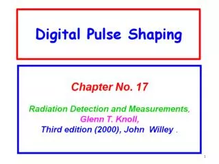
1. Ch 17 GK I Linear and Logical Pulse II Instruments Standard III Application Specific Integrated Circuits IV Summary of Pulse Processing Units V Components common to many applications. VI Pulse Counting Systems

E N D
Ch 17 GK I Linear and Logical Pulse II Instruments Standard III Application Specific Integrated Circuits IV Summary of Pulse Processing Units V Components common to many applications. VI Pulse Counting Systems VII Pulse Height Analysis VIII Digital Pulse Processing A. Analog-to-Digital Converters B Digital Shaping or Filtering C. Pulse Shape Analysis D. Digital Baseline Restoration E. Deconvolution of Piled-Up Pulses IX System Involving Pulse Timing a) Time Pick off methods b) Measurements of Timing Properties c) Modular Instruments for Timing Measurements X Pulse shape discrimination
8-9: Figure 17.33a shows the architecture of a module that carries out one stage of the process described above. • At each clock cycle, the input voltage is momentarily held by a track-hold (T /H) circuit. • A flash ADC carries out a digitization to n bits (n = 3 in the example above), and that value serves as the digital output of the stage. • That same value is supplied to a digital-to-analog converter (DAC) and subtracted from the input voltage. The analog difference is sent through an amplifier with gain of G corresponding to the magnification factor (G = 8 in the example above), and the amplified analog voltage is passed on to the next stage. • A number of such modules can now be combined in a "multipass" or "pipelined" arrangement illustrated in Fig. 17.33b, with all stages synchronized by a common clock. • The digital outputs of all the modules are combined in a logic block that typically includes functions of bit alignment, error correction, and self-calibration to form the overall digital result. • Because of the serial operation of the individual stages, the final result is produced a number of clock cycles following the appearance of the corresponding analog input. • This "latency time" is the same for all samples and introduces some delay. between input and output, but it does not affect the frequency of the conversions. • Examples of some representative commercially available multipass or pipelined ADCs are given in Table 17.2. • Units have been developed with resolutions of up to 16 bits and with conversion frequencies of up to a few hundred MHz. . It Digital Shaping or Filtering
1. LINEAR TIME-INVARIANT FILTERS-8-10 The processes of shaping the signal pulse from a radiation detector can be thought of as a filtering operation. For example, we have seen that the CR differentiator is equivalent to a high-pass filter in the frequency domain. Most (If the puIs" shxping op.-!ra'ions involve what are known as "linear time-invariant filters." Their definition incorporates the restriction that the properties of the filter are fixed and do not change with time. A "transversal filter“ or "finite impulse response" filter is, by definition, limited to using input data over the restricted time range L < t < 0, where L is the length of the filter. This time range reaches backward from the present time simply because only data that have already occurred can contribute. to the output at a specific instant. The mathematical expression of the filtering process then takes the form of the convolution integral Set) = It vet') H(t - t') dt' (17.26) t - L where H(t) is called the impulse response function of the system. This function reflects the operations carried out by the analog shaping networks in conventional linear amplifiers. The definitions given above apply to cases in which the input data appear as an analog or smoothly varying function. That would be the case if we were dealing with the standard analog voltage output produced by a radiation detector. However, the fast digital converters described in the previous section Can be applied to convert voltage into a series of digital samples. Once this conversion to digital data it is then possible to apply digital, rather than analog, filtering techniques to carry shaping of these pulses.
8-11: For the digital case, we start by assuming that the input signal has been sampled series of values Veil that starts at i = O. The time period between each sequential i simply represents the sampling period of the ADC. For the filtering process, the lent of the impulse response function now becomes a discrete set of weighting H(O) ., . H(L). We will assume that this filter is of finite length L so that the values of are 0 for values of i < 0 or i > L. The convolution process equivalent to Eq. (17.26) then can be written i=j S(j) = 2: V(i)H(j - i) (17.21 i=j-L where S(j) now represents the discrete series of output values produced by the digital fiiltering process. To give a more graphic picture of this filtering process, let us choose an examaple,,‘ which the filter consists of four weighting factors, H(O) ... H(3), so the length of the filter' . is equal to 3. Values of H{i) are by definition 0 outside this range. The input consists of .'~.'.'.' digital samples Veil, where we assume that the data begin at i = O. Evaluating the sum giv ,. in Eq. (17.27) for this example then gives, starting with the first nonzerO output value (j = tJ <04. The process continues producing output values for each succeeding value of j, the numbei~ of terms in the summation reaching four at j = 3, and remaining at four for all higher values of j until the end of the input data sequence is approached.
8-12: This convolution process is illustrated graphically in Fig. 17.34. For the example shoWll the weighting factors are written along the upper line in sequence from right to left. []Qfl H(2) I H(I) I H(O) I I V(O) I V(I) I V(2) I V(3) I V(4) I V(S) I S(O) ., V(O)H(O) I H(3) I H(2) I H(I) I H(O) I I V(O) I V(I) I V(2) I V(3) I V(4) I V(S) I 5(1) ., V(O)H(l) + V(l)H(O) I H(3) I H(2) I H(I) I H(O) I I V(O) I V(l) I V(2) I V(3) I V(4) I V(S) I S(2) = V(O)H(2) + V(I)H(l) + V(2)H(0) Figure 17.34 An illustration of a digital transversal filter. The filter elements are shown (right to left) along the top line of each step, with the digitized data along the lower line. The output is formed by multiplying factors that are aligned and summing. Directly below, the sampled input values are written starting at V(O). The output is then given by multiplying each of these input voltages by the weighting factor shown directly above it and summing over the length of the filter. The first nonzero value of the output occurs for the example of j == O. Each successive value of the output is obtained by displacing the string of input values one step sequentially to the left and again carrying out the multiplication and summation. This process can be visualized as "pulling" the set of weighting functions through the sequence of input data (or "pushing" the data through the filter), advancing one step at a time to produce the sequential output values. When the filter is well past the start of the input data, each output value consists of the sum of four terms, and only the input data that are within three steps of the most recent da!Ji- point being processed contribute to the output at that corresponding point. . Simple transverse filters can easily carry out the basic pulse shaping steps of differentiation and integration. They can also be combined in more complex ways to produce triangular, trapezoidal, or other useful shapes. 46,47 These shaping filters share the common property that they simply implement a series of digital weighting factors that remain perfectly stable unless intentionally changed. The time required to carry out the digital operations is short enough so that these schemes can be implemented on a pulse-by-pulse basis in real time, in much the same manner as analog shaping.
2. ADAPTIVE FILTERING-8-13 Digital pulse-processing systems, since they are controlled through software, easily allow the filter weighting functions to be customized to suit the circumstances of the measurement. In our previous discussion of pulse shaping, it was illustrated that each particular shaping choice results in a somewhat different theoretical signal-to-noise ratio (see Fig. 17.15). The choice of the optimum shaping method depends on the magnitude and nature of the noise that is present with the signal. Systems have been designed48- 51 that sample the detailed character of the noise present with the signal and then choose a weighting function that is optimal for the measured results. This is one . . r xp . . adjust the shaping parameters. Another example of adaptive filtering is applied to systems in which the counting rate changes substantially during a measurement. In many cases, one would like to use shaping methods that lead to wider pulses at low counting rates than can be tolerated at high counting rates as a result of excessive pile-up. An adaptive filtering approach that changes the width of the shaping function as a function of counting rate can adjust automatically to these changing conditions.
I, Pulse Shape Analysis 8-14 Once the input waveform from the detector has been digitized, measurements of its detailed shape also become straightforward. We have seen many examples of detectors in which the detailed time profile of the current pulse reveals additional information about the nature of the event in the detector. Examples are in distinguishing one type of radiation from another, measuring the spatial position of an event, or distinguishing pulses that arise from multiple gamma-ray interactions from those that are due to a single interaction only. Sophisticated algorithms can be used to inspect the string of digital data representing each individual pulse so that rather subtle differences among them can be distinguished. As these operations become more complex, however, it is increasingly difficult to carry them out entirely in real time at high counting rates because of the limited time available between signal pulses. In such cases, the digital data can be sent to memory and the processing completed off-line after the measurement.
D. Digital Baseline Restoration-8-15 In digital pUlse-processing systems, the baseline restoration process described on be accomplished by digitally sampling the baseline between pulses and then appropriate value from the measured pulse amplitude.52 Independent baseline can be obtained for each pulse that is processed or, alternatively, a common applied to a series of pulses between more widely spaced samples of the baseline. one would like multiple digital measurements of the baseline to be taken for a sample to enhance its accuracy, requiring a relatively long time interval between Long intervals occur less frequently than short ones, so there must be a trade-off the accuracy of the baseline measurement and the frequency with which they can be Digital filters that can be applied to these baseline samples to optimize the lllt:aSllrem accuracy are described in Ref. 53. E. Deconvolution of Piled-Up Pulses The availability of digital pulse-processing systems opens the possibility of doing m· than simply tolerating the losses associated with pile-up. If a detailed digital samplin made of each output pulse shape from a pulse processing system, it should in principl possible to distinguish those that originate from a single event from those involving up in which more than one event have contributed. The possibility then arises of dec volving the piled-up pulses into their separate components through a detailed analysis their shape . . Figure 17.35 shows an example of a piled-up pulse, sampled at 10 ns intervals, that actu~ ally arises from two events in the detector. Since the shaping process produces pulses ofifJ predictable shape when operating on isolated single events, piled-up pulses depart fr~ this simple profile and can therefore be selected for further analysis. Combinations of th. ·.]'.' expected shape from two events with varying amplitude and time spacing can be fitted ( the observed pulse shape, following an iterative process. Once the optimal fit is obtain,:~ then the individual amplitudes of each event are obtained from the parameters of the fi~~ and the mutual interference of the two events is eliminated. Not only is the correspondinf; distortion removed from the recorded pulse height spectrum, but now the full informatiom! -100 500 1000 Time(ns) 1500 2000
8-16: Figure 17.35 Demonstration of the deconvolution of piled-Up pulses from the output of a scintillation counter. The sampled data from the ADC operating at 100 MHz are shown as the series of points in both plots. In the bottom plot, an analytic fit to these data using the assumption that a single pulse shape should suffice results in a poor fit. In the top plot, an iterative procedure was used to fit two pulse components that allow the separation of both from the piled-up recorded data. (From Komar and Mak.54) Chapter 17 Systems Involving Pulse TIming 659 carried by the two separated pulses can be obtained. Although the utility of this type of pile-up deconvolution has been demonstrated in off-line systems,54.55 the required processing times are still sufficiently long that it is not yet routine in standard spectroscopy systems in which the pulse analysis is carried out in real time.