Random variables
Random variables. Random variables are extensively used in communication circuits Let the random variable represents the functional relationship between a random variable A and a real number For simplicity the rand variable will be denoted by X

Random variables
E N D
Presentation Transcript
Random variables • Random variables are extensively used in communication circuits • Let the random variable represents the functional relationship between a random variable A and a real number • For simplicity the rand variable will be denoted by X • The random variable can be discrete or continuous
Random variables • The distribution function of the random variable X is given by • Where is the probability taken by the random variable X is less than or equal to a real number x • The distribution function has the following properties
Probability density function pdf • Another useful function relating to the random variable X is the probability density function(pdf)
Probability density function The name density function arises from the fact that the probability of the event equals
Properties of the probability density function The probability density function has the following properties The probability density function is always nonnegative function with a total area of one
Ensemble averages The mean value mx or the expected value of a random variable X is defined by The is called the expected value operator The nth moment of a probability distribution of a random variable X is defined by
Ensemble averages In communication system analysis, only the 1st (n=1) and 2nd (n=2) moment are used When n=1 the mean mx of the random variable can be obtained The mean corresponds to the DC value of a random voltage or current
Ensemble averages When n=2 we obtain the mean square value of the X, as follows
Central moments The central moments are defined as the moments of the difference between random variable X and mx
Second central moment (Variance) and STD The second central moment, called the variance of X which is defined The variance of X is also denoted by and its square root, , is called the standard deviation of X
The variance effect on pdf The variance is a measure of randmoness of the random variable X By specifying the variance of a random variable, we are constraining the width of its probability density function
Relation between variance and the mean square value The variance and the mean square value are related by Thus the variance is the difference between the mean square value and the square of the mean
Random process The random process is a function of two variables: an event A and time
Statistical averages of a random process Because the value of a random process at any future time is unknown, a random process whose distribution functions are continuous can be described statistically with a probability density function In general the probability density function will be different for different times
Statistical averages of a random process Therefore it will be impractical to determine the pdf of a given random process empirically However, a partial description consisting of the mean and the autocorrelation function will be sufficient for the needs of communication function The mean of the random process X(t) is
Statistical averages of a random process Where X(tk) is the random variable obtained by observing the random process at time tk and the pdf of X(tK) PxK(X) is the probability density function over the ensemble of events at time tk
Autocorrelation definition The auto correlation function of a random process X(t) is defined as X(t1) and X(t2) are random variables obtained by observing X(t) at times t1and t2 The autocorrelation function is a measure of the degree to which two time samples of the same random process are related
Stationarity • A random process X(t) is said to be stationary if none of its statics are affected by a shift in the time origin • A random process is said to be a wide sense stationary (WSS) if its mean and its auto correlation do not vary with a shift in the time origin • =a constant
Autocorrelation of a wide sense stationary random process For a wide sense stationary process, the autocorrelation function is only a function of the time difference For a zero mean WSS process, indicates the extent to which the random values of the random process are statistically correlated
Autocorrelation of a wide sense stationary random process In other words the autocorrelation gives an idea of the frequency response that is associated with a random process If changes slowly as increase from zero to some value, it indicates that, on average, sample values of x(t) taken at and are nearly the same This means that the frequency domain representation of X(t) is low frequency
Autocorrelation of a wide sense stationary random process On the other hand if decrease rapidly as is increased, this means that X(t) changes rapidly with time and therefore X(t) contains higher frequencies
Time averaging and ergodicity When a random process belongs to a special class, known as an ergodic process, its time averaging is equal to its ensemble averages This means that the statistical properties of the process can be determined by time averaging of a single sample function of the process
Time averaging and ergodicity This means that the mean of the random process can be rewritten as The auto correlation now can be rewritten as
Time averaging and ergodicity Since time averages equal to ensemble averages for ergodic processes, fundamental electrical engineering parameters, such as DC vlaue, rms value, and average power can be related to the moments of an ergodic random process
Power spectral density and Autocorrelation of a random process A random process can generally be classified as a power signal having a power spectral density (PSD) is particularly useful in communication systems, because it describes the distribution of signal’s power in frequency domain The PSD enables us to evaluate the signal power that will pass through a network having a known frequency characteristics
Features of the PSD functions The PSD enables us to evaluate the signal power that will pass through a network having a known frequency characteristics and is always real valued for X(t) real valued PSD and autocorrelation for a Fourier transform pair Relation between normalized average power and PSD
Meaning of correlation Correlation between two phenomena means how closely do they correspond in behavior or appearance, how well do they match one another An autocorrelation function of a signal describes the correspondence of the signal to itself (in time domain) This can be achieved by producing an exact copy of the signal and located in time at minus infinity
Noise in communication systems Noise is unwanted electrical signals that are always present in electrical systems The presence of noise in communication systems limits the receiver's ability to make correct symbol decision This limits the rate of information transmission
Sources of noise Noise can be generated either by man made sources or natural sources Man made sources include spark-plug ignition noise, switching transients, and other radiating electromagnetic signal Natural noise includes such elements as the atmosphere, the sun, and other galactic sources
Thermal noise One of the noise sources that hard or can not be eliminated even with good engineering design is the thermal or Johnson noise. This type of noise is caused by the motion of electrons in all dissipative components, resistors, wires and so on
Gaussian pdf of thermal noise Thermal noise can be described as a zero mean Gaussian random process which has the following pdf In general a noisy digital bit, can be expressed as the sum of the bit a and the noise n
Gaussian pdf of noisy digital bit The probability density function of the noisy digital bit is given by
White noise The power spectral density of the thermal noise is the same for all frequencies of interest in most communications systems; This means that a thermal noise emanates an equal amount of noise power per unit bandwidth at all frequencies from DC to a bout 1 THz This why this kind of noise is called whit Gaussian noise
PSD of white Gaussian noise The PSD of white Gaussian noise is given by
Autocorrelation of white Gaussian noise The autocorrelation function of the noise is given by the inverse Fourier transform of the noise power spectral density as detailed
Average power in white Gaussian noise The average power of white Gaussian noise is infinte