Download

1 / 16
160 likes | 480 Vues
Statistics The Chi Square Test. Aaed EL- Raba’ai. Introduction (1). We often have occasions to make comparisons between two characteristics of something to see if they are linked or related to each other.

E N D
Statistics The Chi Square Test Aaed EL- Raba’ai
Introduction (1) • We often have occasions to make comparisons between two characteristics of something to see if they are linked or related to each other. • One way to do this is to work out what we would expect to find if there was no relationship between them (the usual null hypothesis) and what we actually observe.
Introduction (2) • The test we use to measure the differences between what is observed and what is expected according to an assumed hypothesis is called the chi-square test.
For Example • Some null hypotheses may be: • ‘there is no relationship between the height of the land and the vegetation cover’. • ‘there is no difference in the location of superstores and small grocers shops’ • ‘there is no connection between the size of farm and the type of farm’
Important • The chi square test can only be used on data that has the following characteristics: The frequency data must have a precise numerical value and must be organised into categories or groups. The data must be in the form of frequencies The expected frequency in any one cell of the table must be greater than 5. The total number of observations must be greater than 20.
χ2 = ∑ (O – E)2 E Formula χ2 = The value of chi square O = The observed value E = The expected value ∑ (O – E)2 = all the values of (O – E) squared then added together
Worked Example • Write down the NULL HYPOTHESIS and ALTERNATIVE HYPOTHESIS and set the LEVEL OF SIGNIFICANCE. • NH ‘ there is no difference in the distribution of old established industries and food processing industries in the postal district of Leicester’ • AH ‘There is a difference in the distribution of old established industries and food processing industries in the postal district of Leicester’ • We will set the level of significance at 0.05.
Table Time! Construct a table with the information you have observed or obtained. Observed Frequencies (O) (Note: that although there are 3 cells in the table that are not greater than 5, these are observed frequencies. It is only the expected frequencies that have to be greater than 5.)
Expected frequency = row total x column total Grand total Now • Work out the expected frequency. Eg: expected frequency for old industry in LE1 = (50 x 13) / 92 = 7.07
(O – E)2 E Now Eg: Old industry in LE1 is (9 – 7.07)2 / 7.07 = 0.53 • For each of the cells calculate.
Check your answers Then Add up all of the above numbers to obtain the value for chi square: χ2 = 15.14.
Finally • Look up the significance tables. These will tell you whether to accept the null hypothesis or reject it. The number of degrees of freedom to use is: the number of rows in the table minus 1, multiplied by the number of columns minus 1. This is (2-1) x (5-1) = 1 x 4 = 4 degrees of freedom. We find that our answer of 15.14 is greater than the critical value of 9.49 (for 4 degrees of freedom and a significance level of 0.05) and so we reject the null hypothesis.
In other words ‘The distribution of old established industry and food processing industries in Leicester is significantly different.’
Short exam: Find chi square , and compare with sig. level 0.01