
Continuous Random Variables and Normal Distributions
E N D
Presentation Transcript
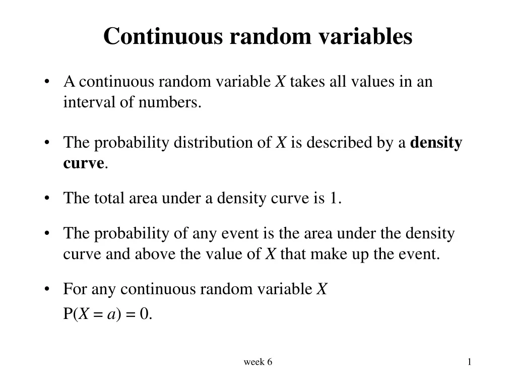
Continuous random variables • A continuous random variable X takes all values in an interval of numbers. • The probability distribution of X is described by a density curve. • The total area under a density curve is 1. • The probability of any event is the area under the density curve and above the value of X that make up the event. • For any continuous random variable X P(X = a) = 0. week 6
Density curves • Density curve is a curve that • is always on or above the horizontal axis. • has area exactly 1 underneath it. • A density curve describes the overall pattern of a distribution. • The area under the curve and above any range of values is the relative frequency (proportion) of all observations that fall in that range of values. week 6
Example: The curve below shows the density curve for scores in an exam and the area of the shaded region is the proportion of students who scores between 60 and 80. week 6
Example – Uniform Distribution • The density function of a continuous Uniform random variable X is given in the graph below. • Find i) P(X < 7) ii) P(6 < X < 8) iii) P(X = 7) iv) P(5.5 < X < 7 or 8 < X < 9) week 6
The median of a distribution described by a density curve is the point that divides the area under the curve in half. A mode of a distribution described by a density curve is a peak point of the curve, the location where the curve is highest. Quartiles of a distribution can be roughly located by dividing the area under the curve into quarters as accurately as possible by eye. Median and mean of Density Curve week 6
Normal distributions • An important class of density curves are the symmetric unimodal bell-shaped curves known as normal curves. They describe normal distributions. • All normal distributions have the same overall shape. • The exact density curve for a particular normal distribution is specified by giving its mean and its standard deviation . • The mean is located at the center of the symmetric curve and is the same as the median and the mode. • Changing without changing moves the normal curve along the horizontal axis without changing its spread. week 6
The standard deviation controls the spread of a normal curve. week 6
There are other symmetric bell-shaped density curves that are not normal e.g. t distribution. • The normal density curves are specified by a particular function. The height of a normal density curve at any point x is given by • Notation: A normal distribution with mean and standard deviation is denoted by N(, ). week 6
In the normal distribution with mean and standard deviation , Approx. 68% of the observations fall within of the mean . Approx. 95% of the observations fall within 2 of the mean . Approx. 99.7% of the observations fall within 3 of the mean . The 68-95-99.7 rule week 6
The distribution of heights of women aged 18-24 is approximately N(64.5, 2.5), that is ,normal with mean = 64.5 inches and standard deviation = 2.5 inches. The 68-95-99.7 rule says that the middle 95% (approx.) of women are between 64.5-5 to 64.5+5 inches tall. The other 5% have heights outside the range from 59.5 to 69.5 inches, and 2.5% of the women are taller than 69.5 . Exercise: 1) The middle 68% (approx.) of women are between ____to ___ inches tall. 2) ___% of the women are taller than 66.75. 3) ___% of the women are taller than 72. Example week 6
The Standard Normal distribution • The standard normal distribution is the normal distribution N(0, 1) that is, the mean = 0 and the sdev = 1. • If a random variable X has normal distribution N(, ), then the standardized variable has the standard normal distribution. • There is no formula to calculate areas under a normal curve. Calculations use either software or a table of areas. The most software and tables calculate one kind of area: cumulative proportions . A cumulative proportion is the proportion of observations in a distribution that fall at or below a given value and is also the area under the curve to the left of a given value. week 6
The standard normal tables • Table IV gives proportions for the standard normal distribution. The table entry for each value z is the area under the curve between 0 and z. • The notation we use to find cumulative probabilities is P( Z ≤ z). • Example: week 6
The standard normal tables - Example • What proportion of the observations of a N(0,1) distribution takes values a) less than z = 1.4 ? b) greater than z = 1.4 ? c) greater than z = -1.96 ? d) between z = 0.43 and z = 2.15 ? week 6
Properties of Normal distribution • If a random variable Z has a N(0,1) distribution then P(Z = z)=0. The area under the curve below any point is 0. • The area between any two points a and b (a < b) under the standard normal curve is given by P(a ≤ Z ≤ b) = P(Z ≤ b) – P(Z ≤ a) • As mentioned earlier, if a random variable X has a N(, ) distribution, then the standardized variable has a standard normal distribution and any calculations about X can be done using the following rules: week 6
P(X = k) = 0 for all k. • The solution to the equation P(X≤ k) = p is k = μ + σzp Where zpis the value z from the standard normal table that has area (and cumulative proportion) p below it, i.e. zp is the pth percentile of the standard normal distribution. week 6
1. The marks of STA221 students has N(65, 15) distribution. Find the proportion of students having marks (a) less then 50. (b) greater than 80. (c) between 50 and 80. 2. Scores on SAT verbal test follow approximately the N(505, 110) distribution. How high must a student score in order to place in the top 10% of all students taking the SAT? 3. The time it takes to complete a stat220 term test is normally distributed with mean 100 minutes and standard deviation 14 minutes. How much time should be allowed if we wish to ensure that at least 9 out of 10 students (on average) can complete it?(final exam Dec. 2001) Questions week 6
General Motors of Canada has a deal: ‘an oil filter and lube job in 25 minutes or the next one free’. Suppose that you worked for GM and knew that the time needed to provide these services was approximately normal with mean 15 minutes and std. dev. 2.5 minutes. How many minutes would you have recommended to put in the ad above if it was decided that about 5 free services for 100 customers was reasonable? 5. In a survey of patients of a rehabilitation hospital the mean length of stay in the hospital was 12 weeks with a std. dev. of 1 week. The distribution was approximately normal. • Out of 100 patients how many would you expect to stay longer than 13 weeks? • What is the percentile rank of a stay of 11.3 weeks? • What percentage of patients would you expect to be in longer than 12 weeks? • What is the length of stay at the 90th percentile? • What is the median length of stay? week 6
Normal quantile plots and their use • If the stem-and-leaf plot or histogram appears roughly symmetric and unimodal, we use another graph, called normal quantile plot as a better way of judging the adequacy of a normal model. • Any normal distribution produces a straight line on that plot. • Interpretation of normal quantile plots: If the points on a normal quantile plot lie close to a straight line, the plot indicates that the data are normal. Systematic deviations from a straight line indicate a nonnormal distribution. Outliers appear as points that are far away from the overall pattern of the plot. week 6
Histogram, the nscores plot and the normal quantile plot for data generated from a normal distribution (N(500, 20)). week 6
Histogram, the nscores plots and the normal quantile plot for data generated from a right skewed distribution week 6
Histogram, the nscores plots and the normal quantile plot for data generated from a left skewed distribution week 6
Histogram, the nscores plots and the normal quantile plot for data generated from a uniform distribution (0,5) week 6
Below are 4 normal probability (quantile) plots and 4 histograms produced by MINITAB for some data sets. The histograms are not in the same order as normal scores plots. Match the histograms with the nscores plots. Question(similar to Q5 Term test Oct, 2000) week 6