Wiggler modeling Double-helix like option

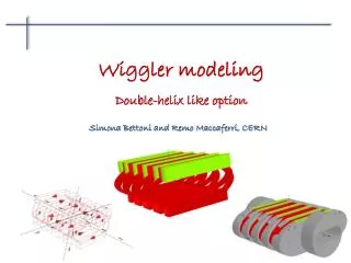
1. Wiggler modelingDouble-helix like option Simona Bettoni and Remo Maccaferri, CERN

2. Outline • Introduction • The model • 2D (Poisson) • 3D (Opera Vector Fields-Tosca) • The analysis tools • Field uniformity • Multipoles (on axis and trajectory) • Tracking studies • The integrals of motion cancellation • Possible options • The final proposal • The prototype analysis • Conclusions

3. Wigglers/undulators model Large gap & long period mid-plane Small gap & short period

4. 2D design (proposed by R. Maccaferri) • Advantages: • Save quantity of conductor • Small forces on the heads (curved part) BEAM

5. The 3D model

6. The 3D model (base plane)

7. The 3D model (extrusions)

8. The 3D model (conductors) Conductors generated using a Matlab script • Conductors grouped to minimize the running time • Parameters the script: • Wire geometry (l_h, l_v, l_trasv) • Winding “shape” (n_layers, crossing positions)

9. The analysis tools • Tracking analysis: • Single passage: ready/done • Multipassage: to be implemented • Field uniformity: ready/done • Multipolar analysis: • Around the axis: ready /done • Around the reference trajectory: ready x and x’ at the exit of the wiggler

10. Prototype analysis z x y

11. Field distribution on the conductors BMod (Gauss) • Maximum field and forces (PMAX ~32 MPa) on the straight part • Manufacture: well below the limit of the maximum P for Nb3Sn • Simulation: quick to optimize the margin (2D)

12. The 2D/3D comparison 1.9260 T 2D (Poisson) -2.1080 T 1.9448 T 3D (Tosca) -2.1258 T

13. Field uniformity (x range = ±2 cm) z (cm)

14. Multipolar analysis (x range = ±2 cm)

15. Multipolar analysis (x range = ±2 cm)

16. Multipolar analysis (x range = ±2 cm)

17. Tracking studies Trajectory x-shift at the entrance = ± 3 cm z x y

18. Tracking studies: the exit position Subtracting the linear part

19. Tracking studies: the exit angle

20. Integrals of motion = 0 for anti-symmetry 1st integral 2nd integral Offset of the oscillation axis CLIC case: even number of poles (anti-symmetric) No offset of the oscillation axis

21. Integrals of motion: the starting point = 0 for anti-symmetry 1st integral 2nd integral (cm)

22. Lowering the 2nd integral: what do we have to do? To save time we can do tracking studies in 2D up to a precision of the order of the difference in the trajectory corresponding to the 2D/3D one (~25 mm) and only after refine in 3D.

23. Lowering the 2nd integral: how can we do? → Highly saturated → → • What we can use: • End of the yoke length/height • Height of the yoke • Terminal pole height (|B| > 5 T) • Effectiveness of the conductors

24. Lowering the 2nd integral: option 1

25. The multipoles of the option 1 Starting configuration (CLICWiggler_7) Modified (option 1) (CLICWiggler_8)

26. Lowering the 2nd integral: option 2 (2D)

27. Option 1 vs option 2 • The “advantage” of the option 2: • Perfect cancellation of the 2nd integral • Field well confined in the yoke • Possibility to use only one IN and one OUT (prototype) • The “disadvantage” of the option 2: • Comments? • The “advantage” of the option 1: • Quick to be done • The “disadvantage” of the option 1: • Not perfect cancellation of the 2nd integral • Field not completely confined in the yoke • Multipoles get worse → start → → → end → 1st layers (~1/3 A*spire equivalent) All the rest

28. Lowering the 2nd integral: option 2 (3D) If only one IN and one OUT → discrete tuning in the prototype model

29. Tracking studies (optimized configuration) Not optimized Optimized

30. Working point: Nb3Sn & NbTi Wire diameter (insulated) = 1 mm Wire diameter (bare) = 0.8 mm Non-Cu fraction = 0.53 Cu/SC ratio = 1 * Nb3Sn NbTi Nb3Sn NbTi *MANUFACTURE AND TEST OF A SMALL CERAMIC-INSULATED Nb3Sn SPLIT SOLENOID, B. Bordini et al., EPAC’08 Proceedings.

31. Possible configurations Possible to increase the peak field of 0.5 T using holmium

32. Working point: comparison

33. Short prototype status & scheduling

34. Conclusions • A novel design for the CLIC damping ring has been analyzed (2D & 3D) • Advantages: • Less quantity of conductor needed • Small forces on the heads • Analysis on the prototype: • Maximum force • Multipolar analysis • Tracking studies • Zeroing the integrals of motion • Future plans • Optimization of the complete wiggler model (work in progress): • Best working point definition • Modeling of the long wiggler • 2nd integral optimization for the long model • Same analysis tools applied to the prototype model (forces, multipoles axis/trajectory, tracking) • Minimization of the integrated multipoles

35. Extra slides

36. Longitudinal field (By = f(y), several x) • Scan varying the entering position in horizontal, variation in vertical: • Dz = 0.1 mm for x-range = ±1 cm • Dz = 2 mm for x-range = ±2 cm

37. Horizontal transverse field (Bx = f(y), several x) • Scan varying the entering position in horizontal, variation in vertical: • Dz = 0.1 mm for x-range = ±1 cm • Dz = 2 mm for x-range = ±2 cm

38. Controlling the y-shift: cancel the residuals W1 W2 W3 W4 W1 W2 W3 W4 2 mm in 10 cm -> 20*2 = 40 mm in 2 m

39. Controlling the x-shift: cancel the residuals (during the operation) To be evaluated the effect of the kicks given by the quadrupoles W1 W2 … Entering at x = 0 cm Entering at x = -DxMAX/2 Entering at x = +DxMAX/2 (opposite I wiggler … positron used for trick)

40. The fit accuracy: an example

41. Field uniformity (x-range = ±3 cm)

42. Multipolar analysis (x-range = ±3 cm)

43. Tracking at x-range = ±3 cm: exit position Subctracting the linear part

44. Tracking at x-range = ±3 cm: exit angle

45. Tracking optimized (x-range = ±3 cm)

46. Holmium option

47. BINP wire

48. 2nd integral optimization (long model)

49. Long wiggler modeling • Problem: very long running time (3D) because of the large number of conductors in the model • Solution: • Build 2D models increasing number of periods until the field distribution of the first two poles from the center give the same field distribution (Np) • Build 3D model with a number of poles Np • “Build” the magnetic map from this

50. Damping ring layout