Algorithms for Formal Circuit Optimization on a Static Timing Basis
730 likes | 916 Vues
Algorithms for Formal Circuit Optimization on a Static Timing Basis. Chandu Visweswariah IBM Thomas J. Watson Research Center Yorktown Heights, NY. Acknowledgments. Partners in crime Andy Conn – Ruud Haring David Ling – Phil Strenski Chai Wah Wu – Ee Cho

Algorithms for Formal Circuit Optimization on a Static Timing Basis
E N D
Presentation Transcript
Algorithms for FormalCircuit Optimization ona Static Timing Basis Chandu Visweswariah IBM Thomas J. Watson Research Center Yorktown Heights, NY
Acknowledgments • Partners in crime • Andy Conn – Ruud Haring • David Ling – Phil Strenski • Chai Wah Wu – Ee Cho • Walt Molzen – Mike Henderson • Katya Scheinberg – Abe Elfadel • Peter O’Brien – Greg Northrop • Pat Williams • several summer students along the way • all the users of our tuners in IBM!
Outline • The benefits of tuning/optimization • Taxonomy • heuristic methods in brief (e.g., TILOS) • Algorithms for formal methods • formulation • incremental sensitivity computation • nonlinear optimization • pruning • optimality conditions • Lagrangian Relaxation (LR) • Methodology implications
Benefits of tuning/optimization • Better circuits • area, delay, power, noise • Enhanced designer productivity • designers’ focus shifts to a higher level like comparing different topologies • Better understanding of tradeoffs • better use of silicon technology • Effective tuning/optimization is an enabler of design for manufacturability • improved parametric yields
Dynamic Static Tuners Heuristic Formal Taxonomy • Today’s tutorial will focus mostly on formal static tuning
Nonlinear optimizer Tuner Simulator Dynamic vs. static tuning • Dynamic tuning is to transient simulation as static tuning is to static timing analysis • examples: DELIGHT.SPICE, JiffyTune • user provides input patterns • user lists paths to be considered • user poses carefully thought-out optimization problem Transistor/wire sizes Function/gradient values
Static tuning • Uses static timing analysis as a basis • All paths through the logic implicitly considered • User does not specify paths or input patterns; easier to use • Inherits weaknesses of static timing analysis • pessimism • false paths • More difficult to include power/noise considerations during tuning
Formal vs. heuristic static tuning • The formal approach attempts to solve the problem “exactly” • better quality of results • long run times • sophisticated mathematical algorithms • significant development effort • The heuristic method repeatedly upsizes the most sensitive transistor(s) on the most critical path(s) • greedy algorithm • generates an area vs. speed tradeoff curve • can handle larger circuits
Heuristic tuning • Example: TILOS (Fishburn and Dunlop, ’85) • Proved that transistor sizing is a convex problem under an Elmore delay assumption • Unfortunately • Elmore delays are too inaccurate • slew effects are not taken into account • meaningful tuning requires additional constraints like slew limits, input loading, ratio constraints which may not be convex • all of these destroy the convexity of the problem • We give up convexity for accuracy
TILOS algorithm • Start all transistors at minimum size • Determine the critical path • Find the sensitivity of the critical path delay to the width of each transistor on the path • Increase width of transistor with highest negative sensitivity by a fixed step size • Repeat • Generates a speed vs. area tradeoff curve • Can consider more than one transistor and/or more than one path at a time
Most critical Next-most critical Comments on heuristic tuning • The answer can be sub-optimal • Can exploit incremental timing algorithms to determine sensitivities by finite differences • Can use more realistic delay models • Difficult to incorporate additional constraints (loading, slew, ratio)
Algorithms for formal static tuning • Goals • obtain an optimal answer (local minimum if problem is not convex) • fully automated solution • take all paths into account • delay calculation using time-domain simulation • flexibility to express wide range of constraints • transistor-level tuner • Components • fast simulation and incremental sensitivity • nonlinear optimization package
Digression: minimax optimization • This problem is not smooth! • Re-map to: • This trick converts a minimax problem into a standard twice continuously differentiable nonlinear optimization problem
Reformulated problem • ATs are variables of the problem • At the solution • original problem is solved because by definition z is minimized and the constraints are feasible • ATs on critical path are correct because these constraints are tight • off-critical ATs may be “wrong” • dij’s are functions of transistor widths • Amenable to addition of any additional general (nonlinear) constraints • slew, input loading, ratio
Constraint generation • Each delay, slew depends on a singleinput slew i j
Simplified view of assertions Combinationalmacro beingtuned Launchinglatch Capturinglatch Primary inputarrival time Primary outputrequired arrivaltime Delaythroughmacro z
Read netlist; create timing graph Formulate optimization problem Feed problem to nonlinear optimizer Snap-to-grid; back-annotate; re-time Solve optimization problem, call simulator for delays/slews and gradients thereof Obtain converged solution Fast simulation and incremental sensitivity computation Components of a tuner
Components of a tuner • Transistor-level static timing analyzer • timing graph, sensitizations, simulation of CCCs, slack calculations • Fast time-domain circuit simulator • Fast time-domain incremental sensitivity • adjoint method • direct method • State-of-the-art nonlinear optimizer • should be able to handle general nonlinear inequalities and objective functions • should be able to handle large problems
Components: fast simulator • Many fast transistor-level time-domain simulators in the literature • orders of magnitude speedup over SPICE • event-driven algorithms • simplified device models (tables for i-v characteristics, simplified parasitic models) • 5% typical, 20% worst-case errors on astage-delay basis • typically invoked via an API by the timer with many “tricks” to ensure efficiency • simulator must handle simulation of CCCs at multiple process corners (best-case, nominal, worst-case)
Accurate gradients indispensable Go West, young man! Mount Elmore Mount Reality
Gradient computation • Direct method • directly differentiate branch characteristics • any number of functions, one parameter • easily extended to the time-domain • Adjoint method • best approached via Tellegen’s theorem • one function, any number of parameters • requires backward-in-time simulation of the adjoint circuit and convolution of waveforms • Either case • take advantage of event-driven paradigm!
Nonlinear optimization • Much progress in nonlinear optimization in the last two decades • A few state-of-the-art packages available • Can solve large problems (50,000 constraints, 50,000 variables) • Can accommodate general nonlinear objective functions and inequality constraints, and simple bounds on variables • Must exploit partial separability (structure) of the problem to render solution practical
Customization of the optimizer • Do not use the optimizer as a black box! • Customization to circuit tuning yields tremendous benefits • Remember: • any simulation-based scheme involves function and gradient data that are numerically noisy • circuit tuning is simulation-intensive; try to reduce the number of iterations • tune the optimizer to be aggressive • gradient computation is expensive • consider adjoint Lagrangian methods • consider reducing the number of variables
Customization of the optimizer • Examples of optimizer customization: • choose tolerances and stopping criteria based on level of noise • methods to reduce numerical noise • failure recovery when the optimizer is too aggressive • “2-step updates” for accelerated convergence • initialization of variables and multipliers • posing of a well-scaled problem; sensible choices of units • reduction of dimensionality of the problem;e.g., treating fanout capacitances as“internal variables” of the optimization
Outline • The benefits of tuning/optimization • Taxonomy • Heuristic methods in brief (e.g., TILOS) • Algorithms for formal methods • formulation • incremental sensitivity computation • nonlinear optimization • pruning • optimality conditions • Lagrangian Relaxation (LR) • Methodology implications
Degeneracy! Springs and planks analogy
Problems with formulation • Size (problem with 2,388 gates has 24,768 variables and 19,175 inequality constraints) • Degeneracy • many equally good solutions since off-critical arrival times and slews can take one of several equally correct values • active (tight) constraints have no impact on the final solution (i.e., their Lagrange multiplier = 0) • Redundancy • many constraints can be removed without changing the solution
Definitions (at the solution) • A “normal” constraint is active and has a unique, non-zero multiplier • A degenerate constraint is active and has a zero or non-unique multiplier • A redundant constraint can be removed without changing the solution; it has a unique, zero multiplier, but may or may not be active • Note: all active degenerate constraints are redundant; not all degenerate constraints are redundant
1 2 3 4 Pruning: an example • 3 timing variablesinstead of 9 • 2 nonlinear constraintsinstead of (6 nonlinear + 2 linear) constraints
1 2 3 4 3r 4r 1r 2r Sink 3f 4f 1f 2f 1r 2f, 3r, 4f Sink 2r, 3f, 4r 1f Pruning: an example
5 1 4 2 6 3 Block-based Path-based Block-based & path-based timing
1 5 2 6 3 Block-based & path-based timing • In timing graph, if node has n fanins, m fanouts, eliminating it causes mn constraints instead of (m+n) • Criterion: if mn (m+n)+1, prune! • Can take slack variable into account 1 5 4 2 6 3
Pruning strategy • During pruning, number of fanins of anyun-pruned node monotonically increases • During pruning, number of fanouts of any un-pruned node monotonically increases • Hence, if a node is not pruned in the first pass, it will never be pruned, since the chances of it getting pruned monotonically worsen • Therefore, a one-pass algorithm can be used for a given pruning criterion
Three-pass greedy pruning • First pass gain=2, then gain=1, then gain=0 • Not optimal, but yields excellent results
Pruning observations • If either m or n is 1, pruning is good! • Even if a node is pruned, its rising/falling slews continue to be variables • Pruning can be done purely topologically • Duplicating nonlinear elements (the dijs) does not increase simulation run time • Duplicating nonlinear elements does not adversely impact the optimization • the gradient/Hessian of each nonlinearelement is only computed and stored once • Three-pass greedy pruning provides tremendous pruning benefits efficiently
1 7 2 9 11 3 14 15 12 4 16 5 10 13 8 6 Detailed pruning example
Edges = 26 Nodes = 16 (+2) Score Card Detailed pruning example 1 7 9 11 14 2 3 15 12 Sink Source 4 8 10 13 16 5 6
Edges = 26 20 Nodes = 16 10 Score Card 1 2 3 4 5 6 Detailed pruning example 7 9 11 14 15 12 Sink Source 8 10 13 16
Edges = 20 17 Nodes = 10 7 Score Card 14 14 15 16 Detailed pruning example 7 9 11 1 2 12 Sink 3 Source 4 5 8 10 13 6
Edges = 17 16 Nodes = 7 6 Score Card 1,7 2,7 3,7 Detailed pruning example 9 11 14 14 12 Sink Source 15 4 5 8 10 13 6 16
Edges = 16 15 Nodes = 6 5 Score Card 11,14 Detailed pruning example 9 1,7 2,7 14 12 Sink Source 3,7 15 4 5 8 10 13 6 16
Edges = 15 14 Nodes = 5 4 Score Card 13,16 Detailed pruning example 9 11,14 1,7 2,7 14 12 Sink Source 3,7 15 4 5 8 10 6