Supercell storms
Supercell storms. Storm splitting, environmental conditions, propagation. Ordinary/multicell storm. Browning et al. (1976). Fovell and Tan (1998). Supercell (rotating) storm. Plan view at surface UD = updraft FFD = forward flank downdraft RFD = rear flank downdraft Gust front Hook echo

Supercell storms
E N D
Presentation Transcript
Supercell storms Storm splitting, environmental conditions, propagation
Ordinary/multicell storm Browning et al. (1976)
Supercell (rotating) storm Plan view at surface UD = updraft FFD = forward flank downdraft RFD = rear flank downdraft Gust front Hook echo Dot ~ tornado location Lemon and Doswell (1979)
Beneath a rotating supercell Made using ARPS and Vis5D
Storm splitting Wilhelmson and Klemp (1981)
Storm splitting (delcity_str_Vprt_QR.MOV) Two symmetric storms result from initial impulse Yields right & left movers Note rotation Domain is moving to east; storm motion subtracted Made w/ ARPS and Vis5D
24 April 2007 splitting storm(as seen from Laughlin AFB radar in SW Texas)
Split L mover weaker R mover turns right R mover hook Purple = hail
Tornado report Maverick, TX
Dynamics of storm splitting Klemp (1987); See Houze p. 288-295
…leads to splitting and rotation Lifting of vortex tubes by updrafts create counter-rotating horizontal vortices… vertical vorticity Low pressure in the vortices establish new updrafts on original storm’s flanks The original storm decays… and voila, the storm appears to have split, yielding counter-rotating storms Note now L pressure and updraft are colocated… shear has contributed to storm stabilization
Precipitation is NOT involved Simulations without rain still show storm splitting
Close look at two papers • Weisman and Klemp (1982) • Environmental conditions favoring ordinary/multicell storms and supercell storms • Rotunno and Klemp (1982) • Why right-movers are favored in U.S. • Why right-movers move to right of mean winds
Weisman and Klemp (1982; “WK”) • “Dependence of Numerically Simulated Convective Storms on Vertical Wind Shear and Buoyancy” • 3D simulations, started with thermal • Varied CAPE by manipulating boundary layer moisture • Considered speed shear only see Houze, p. 284-288
CAPE • Convective Available Potential Energy • “positive area” of a sounding • Integrated from LFC to EQL • WK and Houze (eq. 8.1, p. 283) expressions involve potential temperature • Should involve virtual potential temperature
WK’s sounding CAPE varied by setting PBL moisture Standard case has 14 g/kg
WK wind profiles Us = wind speed change over 10 km Note: no directional shear
WK Wmax vs. time q = 14 g/kg simulations No shear case: intensifies fastest dies first Larger shear - slower development By this metric, moderate shear storm is strongest
WK simulations have symmetry axis No initial flow in N-S direction; Initial bubble is radially symmetric. Therefore, storms have N-S symmetry
WK results multicellular supercellular
Us = 30 m/s, q = 14 g/kg Surface rainwater (g/kg) and surface positive vorticity (1/s, dashed) Low-level radar reflectivity field BWER = Bounded weak echo region
“Secondary storms” are Subsequent ordinary cell developments (i.e., multicells) “Split storms” are supercells, resulting from splitting of initial cell
WK analysis “Bulk Richardson number” ∆u = avg. wind of lowest 6 km minus avg. wind of lowest 500 m “Storm strength” Wmax = largest updraft Denominator = theoretical updraft max ~ ignores pressure perturbation!
WK analysis Larger BRi = initial storm stronger • more CAPE, or • less shear Largest is ~ 60% of theoretical max Multicells favored for BRi > 30 or so… Supercells • smaller BRi • relatively larger S R = BRi
Concerns w/ BRi • CAPE • As formulated in WK (and Houze’s eq. 8.1), moisture in environment neglected (apart from parcel definition) • Water loading, entrainment neglected • Convective inhibition (CIN) completely ignored • Shear • Relevant depth 6 km? Always? • Directional shear completely ignored • Uniqueness of BRi • Same value for low CAPE/low shear as high CAPE/high shear. Reasonable to expect same convective mode and/or intensity? • This has been a very valuable result
Rotunno and Klemp (1982; “RK”) • Most tornadoes associated with supercells • tornadoes have same sense of rotation as parent storm • Further, vast majority of tornadoes are CCW rotating • after splitting, CW left movers tend to die (and/or be non-tornadic) • So why are left movers disfavored? • it’s directional vertical shear
Straight vs. curved hodograph Note mirror-image storms; both have hook-like echoes Note only right-mover has hook shape; left-mover weaker
Straight vs. curved hodograph W at 1.5 km Without directional shear, symmetric pulse always remains symmetric With directional shear, right mover soon favored
Pressure decomposition • Recall nondimensional pressure perturbation π’ subdivided into dynamic and buoyancy pressures • Dynamic pressure can be further partitioned into linear (L) and nonlinear (NL) pressures using perturbation analysis NOTE the overbars… the base state winds
π’ caused by vertical shear π’ - heavy contours - thin contours Vertical shear vector shown X-direction:
Propagation to left & right On flanks, both CW & CCW cause L pressure where vort is max, min L L Net result… L pressure on flanks + L pressure ahead lead to propagation to left and right of mean winds
Unidirectional shear case • Vertical accel largest on E (forward) side… storm moves E • Nonlinear p’ encourages ascent on flanks -- storm splitting • Result symmetric (neither split storm member is favored) Shear vector shown
Directional shear case • RK’s analysis shows that pNL and buoy favor the left mover. • But pLfavors the right mover and dominates
• Hodograph with directional shear. Thin shear vector used for lower-level shear. • Circle indicates updraft. • Linear term encourages low pressure downshear; high pressure upshear • For lower-level shear, lowered pressure to NE
• Upper level shear produces pressure perturbations in different places • On south side of updraft there is lowered pressure aloft overlying raised pressure below. This flank is favored for ascent.