TRANSFORMATION OF FUNCTION OF A RANDOM VARIABLE

1. TRANSFORMATION OF FUNCTION OF A RANDOM VARIABLE UNIVARIATE TRANSFORMATIONS

2. TRANSFORMATION OF RANDOM VARIABLES • If X is an rv with cdf F(x), then Y=g(X) is also an rv. • If we write y=g(x), the function g(x) defines a mapping from the original sample space of X, S, to a new sample space, , the sample space of the rv Y. g(x): S 

3. TRANSFORMATION OF RANDOM VARIABLES • Let y=g(x) define a 1-to-1 transformation. That is, the equation y=g(x) can be solved uniquely: • Ex: Y=X-1  X=Y+1 1-to-1 • Ex: Y=X²  X=± sqrt(Y) not 1-to-1 • When transformation is not 1-to-1, find disjoint partitions of S for which transformation is 1-to-1.

4. TRANSFORMATION OF RANDOM VARIABLES If X is a discrete r.v. then S is countable. The sample space for Y=g(X) is ={y:y=g(x),x S}, also countable. The pmf for Y is

5. Example • Let X~GEO(p). That is, • Find the p.m.f. of Y=X-1 • Solution: X=Y+1 • P.m.f. of the number of failures before the first success • Recall: X~GEO(p) is the p.m.f. of number of Bernoulli trials required to get the first success

6. Example • Let X be an rv with pmf Let Y=X2. S ={2,  1,0,1,2}  ={0,1,4}

7. FUNCTIONS OF CONTINUOUS RANDOM VARIABLE • Let X be an rv of the continuous type with pdf f. Let y=g(x) be differentiable for all x and non-zero. Then, Y=g(X) is also an rv of the continuous type with pdf given by

8. FUNCTIONS OF CONTINUOUS RANDOM VARIABLE • Example: Let X have the density Let Y=eX. X=g1 (y)=log Y dx=(1/y)dy.

9. FUNCTIONS OF CONTINUOUS RANDOM VARIABLE • Example: Let X have the density Let Y=X2. Find the pdf of Y.

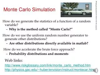
10. THE PROBABILITY INTEGRAL TRANSFORMATION • Let X have continuous cdfFX(x) and define the rvY as Y=FX(x). Then, Y is uniformly distributed on (0,1), that is, P(Y  y) = y, 0<y<1. • This is very commonly used, especially in random number generation procedures.

11. Example 1 • Generate random numbers from X~ Exp(1/λ) if you only have numbers from Uniform(0,1).

12. Example 2 • Generate random numbers from the distribution of X(1)=min(X1,X2,…,Xn) if X~ Exp(1/λ) if you only have numbers from Uniform(0,1).

13. Example 3 • Generate random numbers from the following distribution:

14. CDF method • Example: Let Consider . What is the p.d.f. of Y? • Solution:

15. CDF method • Example: Consider a continuous r.v. X, and Y=X². Find p.d.f. of Y. • Solution:

16. TRANSFORMATION OF FUNCTION OF TWO OR MORE RANDOM VARIABLES BIVARIATE TRANSFORMATIONS

17. DISCRETE CASE • Let X1 and X2 be a bivariate random vector with a known probability distribution function. Consider a new bivariate random vector (U, V) defined by U=g1(X1, X2) and V=g2(X1, X2) where g1(X1, X2) and g2(X1, X2) are some functions of X1 and X2 .

18. DISCRETE CASE • If B is any subset of 2, then (U,V)B iff (X1,X2)A where • Then, Pr(U,V)B=Pr(X1,X2)A and probability distribution of (U,V) is completely determined by the probability distribution of (X1,X2). Then, the joint pmf of (U,V) is

19. EXAMPLE • Let X1 and X2 be independent Poisson distribution random variables with parameters 1 and 2. Find the distribution of U=X1+X2.

20. CONTINUOUS CASE • Let X=(X1, X2, …, Xn) have a continuous joint distribution for which its joint pdf is f, and consider the joint pdf of new random variables Y1, Y2,…, Ykdefined as

21. CONTINUOUS CASE • If the transformation T is one-to-one and onto, then there is no problem of determining the inverse transformation. An and Bk=n, then T:AB. T-1(B)=A. It follows that there is a one-to-one correspondence between the points (y1, y2,…,yk) in B and the points (x1,x2,…,xn) in A. Therefore, for (y1, y2,…,yk)B we can invert the equation in (*) and obtain new equation as follows:

22. CONTINUOUS CASE • Assuming that the partial derivatives exist at every point (y1, y2,…,yk=n)B. Under these assumptions, we have the following determinant J

23. CONTINUOUS CASE called as the Jacobian of the transformation specified by (**). Then, the joint pdf of Y1, Y2,…,Ykcan be obtained by using the change of variable technique of multiple variables.

24. CONTINUOUS CASE • As a result, the function g is defined as follows:

25. Example • Recall that I claimed: Let X1,X2,…,Xn be independent rvs with Xi~Gamma(i, ). Then, • Prove this for n=2 (for simplicity).

26. M.G.F. Method • If X1,X2,…,Xn are independent random variables with MGFs Mxi (t), then the MGF of is

27. Example • Recall that I claimed: • Let’s prove this.

28. Example • Recall that I claimed: Let X1,X2,…,Xn be independent rvs with Xi~Gamma(i, ). Then, • We proved this with transformation technique for n=2. • Now, prove this for general n.

29. More Examples on Transformations • Example 1: • Recall the relationship: If , thenX~N( , 2) • Let’s prove this.

30. Example 2 • Recall that I claimed: Let Xbe an rv with X~N(0, 1). Then, Let’s prove this.

31. Example 3 Recall that I claimed: • If X and Yhave independentN(0,1) distribution, then Z=X/Yhas a Cauchy distribution with =0 and σ=1. Recall the p.d.f. of Cauchy distribution: Let’s prove this claim.

32. Example 4 • See Examples 6.3.12 and 6.3.13 in Bain and Engelhardt (pages 207 & 208 in 2nd edition). This is an example of two different transformations: • In Example 6.3.12: In Example 6.3.13: X1 & X2 ~ Exp(1) Y1=X1-X2 Y2=X1+X2 X1 & X2 ~ Exp(1) Y1=X1 Y2=X1+X2

33. Example 5 • Let X1 and X2 are independent with N(μ1,σ²1) and N(μ2,σ²2), respectively. Find the p.d.f. of Y=X1-X2.

34. Example 6 • Let X~N( , 2) and Y=exp(X). Find the p.d.f. of Y.