Download
1 / 45
450 likes | 539 Vues
Learn about opacity, its wavelength dependency, and how it affects energy flow in stars. Explore sources and key factors influencing opacity in stars, including the formation of absorption lines and continuum spectrum. Gain insights into the physics behind opacity in stellar atmospheres.

E N D
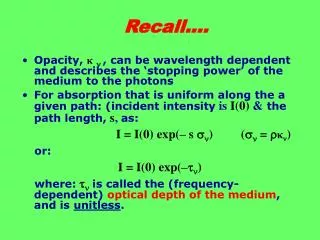
Recall.... • Opacity, κ , can be wavelength dependent and describes the ‘stopping power’ of the medium to the photons • For absorption that is uniform along the a given path: (incident intensity is I(0) & the path length,s, as: I = I(0) exp(–s ) ( = κ) or: I = I(0) exp(–) where:is called the (frequency-dependent) optical depth of the medium, and is unitless.
Overview of Lecture • Equation of Radiative Transfer • Examine what causes opacity in astronomical spectra – in particular in stars. Also examine wavelength dependence • Line formation in stellar atmospheres. Limb-darkening – Source function etc. • Stellar atmospheres: Deviations between real and models – LTE etc.
Interpretation of the equation of radiative transfer • The formal solution of the radiative transfer equation yields the observed intensity of the radiation: • The frequency dependence of the emission and absorption components leads to the formation of emission and/or absorption features.
Optical depth • The overall optical depth of a batch of gas is an important number. If tells us right away if the cloud falls into one of two useful regimes: • optically thin: << 1 • Chances are small that a photon will interact with particle • Can effectively see right through the cloud • In the optically thin regime, the amount of extinction (absorption plus scattering) is linearly related to the amount of material: double the amount of gas, double the extinction • if we can measure the amount of light absorbed (or emitted) by the gas, we can calculate exactly how much gas there is
Optical depth I = I(0) exp(–) I/I(0)= Exp(-10)=5e-5 Exp(-1)=0.37 Exp(-0.1)=0.9 Exp(-0.0001)=0.99 • Optically thick: >> 1 • Certain that a photon will interact many times with particles before it finally escapes from the cloud • Any photon entering the cloud will have its direction changed many times by collisions -- which means that its "output" direction has nothing to do with its "input" direction. Cloud is opaque • You can't see through an optically thick medium; you can only see light emitted by the very outermost layers. • i.e., can’t ‘see’ interior of a star – only see the ‘surface’ or the photosphere • One convenient feature of optically thick materials: the spectrum of the light they emit is a blackbody spectrum, or very close to it layers deep within a star (can assume LTE)
Sources of Opacity • So, if the inner layers of a star can be approximated by a BB, what are the causes of opacity in the outer layers? • Detailed calculation of opacity, κ, is tough and complex problem Major Codes Required! • The wavelength dependence shapes the continuous spectrum emitted by a star. • Major influence on the temperature structure of an atmosphere because the opacity controls how easily energy flows at a given wavelength. • Where opacity is high, energy flow (flux) is low.
Sources of Opacity • Opacity a function of composition, density & temperature. • Determined by the details of how photons interact with particles (atoms, ions, free electrons). • If the opacity varies slowly with λ it determines the stars continuous spectrum (continuum). The dark absorption lines superimposed on the spectrum are the result of a rapid variation of opacity with λ. • Can be broken down into 5 main sources
Sources of Opacity • 5 primary sources of opacity: • Bound-Bound absorption Small, except at those discrete wavelengths capable of producing a transition. i.e., responsible for forming absorption lines – also can form pseudo-continuum at low R • Bound-Free absorption Photoionisation - occurs when photon has sufficient energy to ionize atom. The freed e- can have any energy, thus this is a source of continuum opacity • Free-Free absorption (Bremsstrahlung) A scattering process. A free electron absorbs a photon, causing the speed of the electron to increase. Can occur for a range of λ, so it is a source of continuum opacity. Only important at high temperatures as need lots of free e-. • Electron scattering (Thomson scattering) A photon is scattered, but not absorbed by a free electron. A very inefficient scattering process only really important at high temperatures where it dominates as other as other sources decrease. • Dust extinction Only important for very cool stellar atmospheres and cold interstellar medium more important at short wavelengths, will not treat in this course!
Examples: • Bound-Free absorption: e.g., the Balmer jump or Balmer decrement, the Lyman limit i.e., Structure of the H atom produces spectral features
Examples: • Bound-Bound absorption: e.g., H absorption (Lyman, Balmer, Paschen series etc.), Fe line-blanketing, molecular etc., millions of lines for cooler gas……. Modelled opacity in the UV due to gas at 5,000K (black) and 8,000K (red). The opacities are due to lines, mostly HI, FeII, SiII, NI, OI and MgII Balmer series b-b transitions (note the Balmer edge continuous, so bound-free!)
Mean Opacity All 4 opacities can be grouped to form a mean opacity at a specific wavelength: If we average over all wavelengths we get the ‘Rosseland Mean Opacity’: • Bound-bound term requires millions of transitions (i.e. opacity project) • Bound-free term reasonably approximated by ~T-3.5 • Free-free term ~T-3.5 also • Electron scattering term simply independent of wavelength Contributions to mean opacity with T (at constant density)
Sources of Opacity • Primary sources of opacity in most stellar atmospheres are: • Photoionisation of H- ions, but these become increasingly ionised for stars hotter than the sun, where photoionisation of H atoms and free-free absorption become the main sources. • For O stars the main source is electron scattering, and the photoionisation of He also contributes. Also bound-bound transitions in the UV important – actually can drive wind. • Molecules can survive in cooler stellar atmospheres and contribute to bound-bound and bound-free opacities. The large numbers of molecular lines are an efficient impediment to the flow of photons.
Optical Depth Effects in Stellar Atmospheres:Two examples:1. Line Formation2. Limb-darkening
Optical depth and spectral line formation • Remember that can only ‘see’ a MFP into a cloud (or star) if it is optically thick so, the lower the optical depth, the deeper into the star we see • For weak lines (lower optical depth) the deeper the line formation region • For strong lines (higher optical depth), the shallower the line formation region think of case of cloud in earth’s atmosphere Temperature structure of solar atmosphere
Optical depth and spectral line formation • Formation of absorption lines on the Sun τincreasing
Optical depth and spectral line formation • Formation of absorption features can also be understood in terms of the temperature of the local source function decreasing towards the line centre Limb darkening can be understood in a similar way…
Limb Darkening The sun redder at the edges, also dimmer at the edges…
Limb Darkening Can also be understood in terms of temperature within the solar photosphere. Deeper hotter. Since we ‘see’ ~ 1 optical depth into atmosphere => can see different depths across solar disk • At centre see hotter gas than at edges • Similar effect to line formation earlier • Centre appears hotter, brighter • Limb darkening!
Limb Darkening Variation of intensity across solar disk See notes for further details
Limb Darkening Also see limb darkening in other stars, i.e., red supergiant Betelgeuse – few pixels across!
Thermodynamic equilibrium • If we assume that all the constituents of the gas in a body are in the most probable macrostate (due to random collisions) i.e., they are in (strict) thermodynamic equilibrium • The gas can then be described with a single parameter – the temperature, T,and this same temperature also describes the radiation field • Since system is in equilibrium: • This is true where collisions occur within a volume where the state variables (specifically the temperature) can be considered constant • example: the deep interior of a star
Local Thermodynamic Equilibrium • Nearer the surface, the assumption of thermodynamic equilibrium is only partly true: • mean free path for photons is long, so they “see” the stellar boundary • mean free path for particles is short, so they can be very close to the boundary and yet still act as if they are in equilibrium i.e., they still obey the Maxwell-Boltzmann distribution • Away from the boundary, where the mean free path for photons << thermal scale height, local thermodynamic equilibrium (LTE) is satisfied and we have:
Local Thermodynamic Equilibrium • The assumption of LTE is appropriate if collisional processes amongst particles dominate the competing photoprocesses, or are in equilibrium with them at a common matter and radiation temperature • For gaseous nebulae, interplanetary, interstellar or intergalactic media non-LTE processes are important: • gas is optically thin • photoexcitation is important • Particle density low (few interactions)
Radiation and equilibrium • For a perfect absorber of radiation, the emitted radiation is described by the Planck equation for blackbody radiation at the gas temperature, T: • This equation is important for the derivation of stellar atmospheric properties. In general terms, when material is in thermodynamic equilibrium it is in mechanical, thermal, and chemical equilibrium.
Source function and Kirchoff’s Laws • Given: • This equation can be simply integrated to give: • Two important limits: τ<< 1 andτ>> 1
Source function and Kirchoff’s Laws • For τ<< 1 we can simplify: • So the emission increases with path length (recall that optical depth = σ s) • i.e., emission lines from solar corona at eclipse (so background source)
Source function and Kirchoff’s Laws • For τ>> 1 we can simplify: • So the emission has a constant value Question: how far into the source do we see? Hint: think about the definition of Sυ
Kirchoff’s Laws • Bunsen, Kirchoff (1859) • The three basic types of spectra: • continuum • emission • absorption Think about the application of radiation transfer to these cases (hint: identify source and absorber)
Blackbody spectra Recall the shape of the blackbody curve – this is the limiting emission that an optically thick medium will reach for that temperature
Thermalisation • Consider a uniform slab of gas of thickness L and temperature T that radiates like a blackbody, with an absorption coefficient συwhich is small everywhere except at a strong line of frequency υ0 • Compare the emitted intensity in the line relative to the neighbouring continuum for different limiting optical thicknesses of the slab
Thermalisation • For a gas in TE we have: • and, for frequencies which are similar: • we now have three interesting cases, depending on the balance of the optical depths (absorption cross-sections)
Thermalisation • Case I: medium optically thin for all frequencies – • Case II: line is optically thick, but continuum isn’t - • Case III: medium is optically thick at all frequencies -
Approach to thermalisation Blackbody curve ~ 0 small large very large Approach to thermalisation – line and continuum changes
Scattering • Scattering may be either: • frequency dependent • e.g., line scattering • frequency independent • e.g., scattering by free electrons • If scattering is independent of frequency it is said to be “grey”
Example: Electron scattering es = Thx column density • For electron scattering we have: where: Th is the Thomson cross-section: • Note: The optical depth (amount of scattering) is directly proportional to the number of electrons along the line-of-sight Th = 6.652 x 10⁻²⁵ cm2
Model Atmospheres • Model atmospheres are the key to interpreting observations of real stars • By definition, most of stellar photons we receive are from ‘photosphere’ ( optical depth 2/3 at 500nm) • Need to model in order to compare with observations • Initial model constructed on the basis of observations & known physical laws. • Then modified and improved iteratively until good match achieved. Can then infer certain properties of a star: • temperature, surface gravity, radius, chemical composition, rate of rotation, etc as well as the thermodynamic properties of the atmosphere itself.
Model Atmospheres • A number of simplifications usually necessary!: • Plane-parallel geometry making all physical variables a function of only one space coordinate • Hydrostatic Equilibrium no large scale accelerations in photosphere, comparable • to surface gravity, no dynamical significant mass loss • No fine structures such as granulation, starspots • Magnetic fields are excluded
Stars as Black Bodies? Thermal Equilibrium? • Basic condition for the BB as emitting source negligible fraction of radiation escapes! • Below the lower photosphere optical depth to the surface is high enough to prevent escape of most photons. They are reabsorbed close to where they were emitted - thermodynamic equilibrium - & radiation laws of BB apply. • However, a star cannot be in perfect thermodynamic equilibrium! That would imply no net outflow of energy! • Higher layers deviate increasingly from BB as this leakage becomes more significant. There is a continuous transition from near perfect local thermodynamic equilibrium (LTE) deep in the photosphere to complete nonequilibrium • (non-LTE) high in the atmosphere.
Stars as Black Bodies? Thermal Equilibrium? • Thermodynamic Equilibrium is applied to relatively small volumes of the model photosphere - volumes with dimensions of order unity in optical depth LTE • The photosphere may be characterized by one physical temperature at each depth. • (L)TE means atoms, electrons & photons interact enough that the energy is distributed equally among all possible forms (kinetic, radiant, excitation etc), and the following theories can be used to understand physical processes: • Distribution of photon energies: Planck Law (Black-Body Relation) • • Distribution of kinetic energies: Maxwell-Boltzmann Relation • • Distribution among excitation levels: Boltzmann Equation • • Distribution among ionization states: Saha Equation So one temperature can be used to describe the gas locally
Stars as Black Bodies? Thermal Equilibrium? • So LTE usually assumed works for non-extreme conditions • Often poorly describes very hot stars (strong radiation field) and very extended stars (low densities, i.e., red giants) • Sometimes LTE works for some spectral features, but not for other features in the same star (different lines formed in different regions of photosphere) • Generally models can re-produce stellar spectra very well….
Notes for lectures 3+4: • http://www.maths.tcd.ie/~ccrowley/Astro_spec_lecture_3_4.ppt • http://www.maths.tcd.ie/~ccrowley/Astro_spec_notes_3_4.doc