Improving Neutron Beta Decay Measurements Through Optimized Electron Collimators
This project focuses on refining the measurement of the “a” coefficient, which describes the angular correlation in neutron beta decay involving antineutrinos and electrons. Current measurements have a significant error margin, and this work aims to design and test novel electron collimators to minimize scattering, thereby reducing errors to under 1%. We will investigate the impact of different materials and configurations of collimators, analyzing parameters like scattering ratios to determine optimal designs for precise measurements aligned with the Standard Model.

Improving Neutron Beta Decay Measurements Through Optimized Electron Collimators
E N D
Presentation Transcript
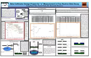
Anti-neutrino Proton and its Helical Path Proton Detector Electron Detector Neutron Electron and its Helical Path Electron helical path Z - axis Random Source Washer Collimator 2 cm Z - axis Side View Random Source 39.4 cm Washer collimator 15.2 cm Electron Detector 2 cm 14.2 cm 0.2 cm 15.2 cm Aluminum Wall Side View Electron helical path 0.2 cm 1 cm 54.6 cm 1 cm 1 cm 15.2 cm Washer Collimators 0.2 cm 3-D View 3-D View 14.2 cm washer collimator 2 mm Electron Detector Electron Detector DUNPL Beta Collimator Design Project for “a” Measurement in Free Neutron Beta DecayAung Kyaw Sint, Travis Clark, Dr. Alexander Komives Test on Collimator Material Collimator Number Test Abstract: Neutron decay has been studied in the past century and several coefficients describing this process have been determined recently. One of these coefficients is called little “a” and is related to the probability the antineutrino and electron from a neutron decay have the same general direction. The previous measurements of “a” contain a total error of about 4%1,2. An experiment that employs a novel method, shown in Figure 1, of measuring this coefficient is now being built3. This new design will reduce the error to less than 1%, allowing us to test the current prediction made by the Standard Model more precisely. The immediate goal of this project is to design electron collimators that will minimize electrons that scatter from the collimator into the electron detector. These events, left unchecked, will cause a large systematic error in “a”. The best collimator configuration (material, number of collimators, collimator shape) is determined by minimizing the ratio R, where Nae is the number of electrons scattered from a collimator into the detector and Nd is the total number of electrons detected. To achieve a sub-1% measurement of “a”, R must be less than 0.003. In order to find out the best material to use, the ratio R was evaluated for a variety of elements, aluminum (Z=13), lead (Z=82), tungsten (Z=74), cobalt (Z=27) and iron (Z=26) as shown in Table 1. As can be seen, iron is marginally better than tungsten or cobalt. Another parameter we wanted to investigate is the number of collimators. We kept other variables (electron energy, thickness, material and collimator shape) the same. Figure 6 has the geometry of 2, 3 and 5 tungsten collimators. We spaced out the distance between collimators equally. We wanted to maintain the spacing between collimators, so we moved the detector further down from the 2 and 3 collimator configuration so we could have 5 collimators. Table 2 recapitulates the results we got from using different numbers of collimators. Electron Collimators One of the most important things that we learned from looking at different numbers of collimators is that the more collimators, the better the ratios become. Also, we discovered a new type of anomalous events happening in 2 collimators. In 1 collimator, we only have side hits. An example of a side hit is shown in Figure 8. When we got to 2 collimators, we found “Act of God” (AOG) events where an electron bounces between the surfaces of two adjacent collimators and eventually makes it into the detector. But, we did not see any AOG’s in 3 collimators and more. Figure 9 has an example of an AOG event. We think that in 3 collimators, although AOG’s could happen between the first and second collimators, the chances of AOG’s occurring between the second and third collimator are very, very small. On the other hand, we should not be seeing any AOG’s in 1 collimator because by definition, AOG’s only occur when there is more than one collimator for an electron to bounce between collimator surfaces. As discussed earlier, the more collimators, the better the ratio is. From Table 2, 5 collimators produced 0.2 % ratio, which is what we want. Notice that it took about 1600 computer hours to get that low ratio. A big leap from 0.05 ratio of 2 collimators to 0.007 ratio of 3 collimators can be explained by having AOG’s in 2 collimators. Figure 7 shows the ratio for different numbers of washer geometry collimators. Table 1: Results of using different materials with the geometry shown in Figures 3 and 4. Table 2: Different number of collimator washer geometry with 0.2 cm thickness and their respective ratios. Magnetic Field Coils 1Byrne et al., Journal of Physics G, 28, 1325 (2002). 2Stratowa et al., Physical Review D 18, 3970 (1978). 3Wietfeldt et al., submitted to Nuclear Instruments and Methods A. Figure 1: The decay of a free neutron producing a proton, electron and an antineutrino in the proposed apparatus. Initial Test of PENELOPE For our simulation, we used a specific Monte Carlo package called PENELOPE (PENetration and Energy Loss of Positrons and Electrons). Basically the program traces the trajectory of an electron randomly generated in the magnetic field. Using quantum mechanics, PENELOPE randomly decides how an electron interacts with material as it travels in the magnetic field, i.e. whether or not it scatters or experiences Bremsstrahlung radiation by emitting X – rays. We first tested our PENELOPE program before running any simulation for collimator design. We verified the experimental result of range number-distance curves for electrons in aluminum measured by Marshal and Ward4. The results from our simulation are compared with the measurements in Figure 2. Within acceptable error, the two sets of data agree nicely proving that PENELOPE simulation can be used without any doubt. 4J. Marshall, A.G. Ward. Can. J. Research A15, 39 (1937) 5N/A indicates that this information was either lost or deleted. Figure 7: The graph showing different number of collimators vs. scattered ratio from Table 2. Figure 5: The graph showing atomic number vs. scattered ratio from Table 1. Z - axis Random Source Figure 2: The graph showing the number of electrons transmitted varies with Aluminum thickness. Collimator Wall Geometry We just started testing the effects of a cylindrical wall around the collimator as one is required to be used as a vacuum chamber. The geometry design is shown in figure 10. We tested it with the 1 tungsten washer collimator design by adding a 1 cm thick aluminum cylinder. We got the ratio 0.046 0.002. We need to run longer simulation to get enough data to compare without a cylindrical wall. 2 cm 15.2 cm Washer collimator 5 0.2 cm Figure 4 portrays the geometry of a washer collimator, electron detector, and the electron source. When the simulation is running, electrons are released in random directions from random positions inside a disk-shaped source to the electron detector. The magnetic field produced by the coils causes the electrons to follow a spiral path. It is possible for an electron to hit the collimator and scatter into the detector or bounce away from the detector. The program recorded and saved events in which the electron hit the collimator and the detector. We label those events anomalous electrons (a.e.). We do not care about those electrons that hit the collimator and do not make it to the detector. Washer Collimator Geometry 19.5 cm 0.2 cm Washer collimator 4 94.2 cm (for 5 collimators) 54.8 cm (for 1,2 and 3 collimators) 19.5 cm Figure 8: An example of side hit where electron hits the inner surface of collimator Future Work 0.2 cm Washer collimator 3 Electron Detector Although we do not have time to run more simulations, we have some good ideas to get a better collimator design. We need to run with different numbers of iron collimators with 70 degree angle wedge shaped and 2 mm thickness. We could also try new geometry shapes. We have not looked at Bremsstrahlung radiation in our simulation. We need to rerun 5 collimators tungsten washer design with Bremsstrahlung effect to see if we get a different ratio. 19.5 cm Washer collimator 2 0.2 cm 19.5 cm Figure 3: The geometry of the aluminum collimator resembling the shape of a washer. 15.2 cm 14.2 cm Washer collimator 1 0.2 cm Electron Detector Figure 4: The geometry of the random source, washer collimator and detector. Figure 10: The geometry of the source, aluminum collimator and detector. Figure 9: An example of AOG event where electron bounces between surfaces of 2 collimators. Figure 6: The geometry of 1, 2, 3, 4 and 5 tungsten collimators and detector.
![Altitude= [0.2, 4.0km]](https://cdn4.slideserve.com/464372/nasa-s-cloud-absorption-radiometer-dt.jpg)