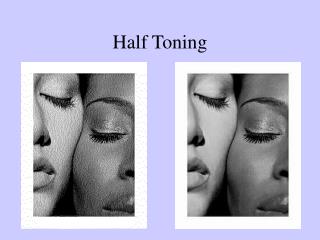
Half Toning
Half Toning. Continuous Half Toning. Color Half Toning. Half toning and Colors. Digital Half Toning. Half Toning. Emulating 5 different levels. Half Toning. 10 levels. Original. Half Toning. Original. Dithering. Dithering and Halftoning. Trade spatial for intensity resolution
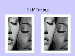

Half Toning
E N D
Presentation Transcript
Half Toning Emulating 5 different levels
Half Toning 10 levels
Dithering and Halftoning Trade spatial for intensity resolution (works well for printing where dot printing is very high) • Thresholding. • Random dither; Robert’s algorithm • Ordered dither • Error diffusion Your eye will average over an area - Spatial Integration
Thresholding Assume we want to quantize a gray-level image to a binary colormap. Map the upper half of the gray-level scale to white, and the lower half to black – a simple threshold operation, preformed independently at each pixel.
Thresholding Simple threshold. Original image. n = 0.5 Errors are low spatial frequencies.
Robert’s Algorithm • First add noise • Then quantize i r + 1 1 Quantized to 1 Quantized to 0 r 0 x Moves errors to higher spatial frequencies. -> eye averages over an area.
Robert’s Algorithm Pink Blue
The trouble with noise • Difficult to compute quickly. • Not reproducible. • Pre-compute pseudo-random function and store in table. • Small tiled patterns sufficient
Dithering • It is possible to improve the quality of a quantized image by distributing the quantized error. • Let’s have a closer look.
Dithering Thresholding Dithering
Dithering Each pixel produces a quatization error The quality of the result may be improved by adjusting the threshold locally, so that adjacent pixels in small areas are quantized with different thresholds. This reduces the average local quantization error. Matrices of these threshold are called dither matrices.
Ordered Dithering • Trade off spatial resolution for intensity resolution. • Use dither patterns. • Can be represented as a matrix.
3 7 5 6 1 2 9 4 8 The dithering matrix (3x3) For all Xpixels For all Ypixels v = approximate(x,y) i = x mod 3 j = y mod 3 if v >= M[i,j] then Set_Pixel(x,y, BLACK) else Set_Pixel(x,y, WHITE)
0 3 0 7 0 5 3 7 7 5 5 8 1 6 2 4 5 3 2 6 0 1 1 2 1 6 6 1 2 8 7 2 2 5 4 3 2 3 9 0 1 4 8 0 4 9 9 4 4 8 8 3 7 5 2 6 4 3 3 7 5 8 9 7 7 2 2 1 3 2 6 6 1 2 2 9 9 7 4 3 2 2 4 8 9 9 4 4 8 8 8 4 4 8 4 4 Dithering 3 7 5 6 1 2 Dithering mask 9 4 8 2 1 3 Image 3 2 2 4 8 4 Binary image
Floyd-Steinberg Error Diffusion With this method, the average quatization error is reduced by propagating the error from each pixel to some of its neighbors in the scan order.
1D Error Diffusion 1 0 1
1D Error Diffusion 1 0 1 0
1D Error Diffusion 1 0 1 0 1
e e -3e/8 -3e/8 -e/4 -3e/8 -e/4 -3e/8 Floyd-Steinberg Error Diffusion With this method, the average quatization error is reduced by propagating the error from each pixel to some of its neighbors in the scan order. Note that the error propagation weights must sum to one
Error diffusion result Dithering result
Dithering Dithering: Note that each square ring is of different brightness
Error Diffusion Error Diffusion: Note that the error is distributed across the layers