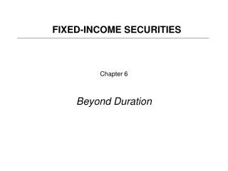
Chapter 6 Beyond Duration

1. FIXED-INCOME SECURITIES Chapter 6 Beyond Duration

2. Outline • Accounting for Larger Changes in Yield • Accounting for a Non Flat Yield Curve • Accounting for Non Parallel Shits

3. Beyond Duration Limits of Duration • Duration hedging is • Relatively simple • Built on very restrictive assumptions • Assumption 1: small changes in yield • The value of the portfolio could be approximated by its first order Taylor expansion • OK when changes in yield are small, not OK otherwise • This is why the hedge portfolio should be re-adjusted reasonably often • Assumption 2: the yield curve is flat at the origin • In particular we suppose that all bonds have the same yield rate • In other words, the interest rate risk is simply considered as a risk on the general level of interest rates • Assumption 3: the yield curve is flat at each point in time • In other words, we have assumed that the yield curve is only affected only by a parallel shift

4. Accounting for Larger Changes in YieldDuration and Interest Rate Risk

5. Accounting for Larger Changes in YieldHedging Error • Let us consider a 10 year maturity bond, with a 6% annual coupon rate, a 7.36 modified duration, and which sells at par • What happens if • Case 1: yield increases from 6% to 6.01% (small increase) • Case 2: yield increases from 6% to 8% (large increase) • Case 1: • Discount future cash-flows with new yield and obtain $99.267 • Absolute change : - 0.733 = (99.267-100) • Use modified duration and find that change in price is -100x7.36x0.001= - $0.736 • Very good approximation • Case 2: • Discount future cash-flows with new yield and obtain $86.58 • Absolute change : - 13.42 = (86.58 -100) • Use modified duration and find that change in price is -100x7.36x0.02= - $14.72 • Lousy approximation

6. Accounting for Larger Changes in YieldConvexity • Relationship between price and yield is convex: • Taylor approximation: • Relative change • Conv is relative convexity, i.e., the second derivative of value with respect to yield divided by value

7. Accounting for Larger Changes in YieldConvexity and $ Convexity • $Convexity = V’’(y) = Conv x V(y) • Example (back to previous) • 10 year maturity bond, with a 6% annual coupon rate, a 7.36 modified duration, a 6974 $ convexity and which sells at par • Case 2: yields go from 6% to 8% • Second order approximation to change in price • Find: -14.72 + (6974.(0.02)²/2) = -$13.33 • Exact solution is -$13.42 and first order approximation is -$14.72 • (Relative) convexity is

8. Accounting for Larger Changes in YieldProperties of Convexity • Convexity is always positive • For a given maturity and yield, convexity increases as coupon rate • Decreases • For a given coupon rate and yield, convexity increases as maturity • Increases • For a given maturity and coupon rate, convexity increases as yield rate • Decreases

9. Accounting for Larger Changes in YieldProperties of Convexity

10. Accounting for Larger Changes in YieldProperties of Convexity - Linearity • Convexity of a portfolio of n bonds where wiis the weight of bond i in the portfolio, and: • This is true if and only if all bonds have same yield, i.e., if yield curve is flat

11. Accounting for Larger Changes in YieldDuration-Convexity Hedging • Principle: immunize the value of a bond portfolio with respect to changes in yield • Denote by P the value of the portfolio • Denote by H1 and H2 the value of two hedging instruments • Needs two hedging instrument because want to hedge one risk factor (still assume a flat yield curve) up to the second order • Changes in value • Portfolio • Hedging instruments

12. Accounting for Larger Changes in YieldDuration-Convexity Hedging • Strategy: hold q1 and q2 units of the first and second hedging instrument respectively such that

13. Duration-Convexity Hedging

14. Solution • Or (under the assumption of a unique y – flat yield curve) • Solution (under the assumption of unique dy – parallel shifts). Find q1 and q2 that solve the linear system in two unknown:

15. Accounting for a Non Flat Yield CurveAllowing for a Term Structure • Problem with the previous method: we have assumed a unique yield for all instrument, i.e., we have assumed a flat yield curve • We now relax this simplifying assumption and consider 3 potentially different yields y, y1, y2 • On the other hand, we maintain the assumption of parallel shifts, i.e., we assume dy= dy1 = dy2 • We are still looking for q1 and q2 such that

16. Accounting for a Non Flat Yield Curve • Solution (under the assumption of unique dy – parallel shifts) • Or (relaxing the assumption of a flat yield curve)

17. Accounting for a Non Flat Yield CurveTime for an Example! • Portfolio at date t • Price P = $ 32863.5 • Yield y = 5.143% • Modified duration Sens = 6.76 • Convexity Conv =85.329 • Hedging instrument 1 • Price H1 = $ 97.962 • Yield y1 = 5.232 % • Modified duration Sens1 = 8.813 • Convexity Conv1 = 99.081 • Hedging instrument 2: • Price H2 = $ 108.039 • Yield y2 = 4.097% • Modified duration Sens2 = 2.704 • Convexity Conv2 = 10.168

18. Accounting for a Non Flat Yield CurveTime for an Example! • Optimal quantities q1 and q2 of each hedging instrument are given by • Or q1 = -305 and q2 = 140 • If you hold the portfolio, you should sell 305 units of H1 and buy 140 units of H2

19. Accounting for Non Parallel ShiftsAccounting for Changes in Shape of the TS • Bad news is: not only the yield curve is not flat, but also it changes shape! • Afore mentioned methods do not allow to account for such deformations • Additional risk factors • One has to regroup different risk factors to reduce the dimensionality of the problem: e.g., a short, medium and long maturity factors • Systematic approach: factor analysis on historical data has shed some light on the dynamics of the yield curve • 3 factors account for more than 90% of the variations • Level factor • Slope factor • Curvature factor

20. Accounting for Non Parallel ShiftsAccounting for Non Parallel Shits • To properly account for the changes in the yield curve, one has to get back to pure discount rates • Or, using continuously compounded rates

21. Accounting for Non Parallel ShiftsNelson Siegel Model • The challenge is that we are now facing m risk factors • Reduce the dimensionality of the problem by writing discount rates as a function of 3 parameters • One classic model is Nelson et Siegel’s • with R(0,): pure discount rate with maturity  • 0 : level factor • 1 : rotation factor • 2 : curvature factor •  : fixed scaling parameter • Hedging principle: immunize the portfolio with respect to changes in the value of the 3 parameters

22. Accounting for Non Parallel ShiftsNelson Siegel Model • Mechanics of the model: changes in beta parameters imply changes in discount rates, which in turn imply changes in prices • One may easily compute the sensitivity (partial derivative) of R(0,) with respect to each parameter beta (see next slide) • Very consistent with factor analysis of interest rates in the sense that they can be regarded as level, slope and curvature factors, respectively

23. Accounting for Non Parallel ShiftsNelson Siegel

24. Accounting for Non Parallel ShiftsNelson Siegel Model • Let us consider at date t=0 a bond with price P delivering the future cash-flows Fi • The price is given by • Sensitivities of the bond price with respect to each beta parameter are

25. Beta 0 Beta 1 Beta 2 Scale parameter 8% -3% -1% 3 Accounting for Non Parallel ShiftsExample • At date t=0, parameters are estimated (fitted) to be • Sensitivities of 3 bonds with respect to each beta parameter, as well as that of the portfolio invested in the 3 bonds, are

26. Accounting for Non Parallel ShiftsHedging with Nelson Siegel • Principle: immunize the value of a bond portfolio with respect to changes in parameters of the model • Denote by P the value of the portfolio • Denote by H1, H2 and H3 the value of three hedging instruments • Needs 3 hedging instruments because want to hedge 3 risk factors (up to the first order) • Can also impose dollar neutrality constraint q0H0 + q1H1 + q2H2 + q3H3 + q4H4 = - P (need a 4th instrument for that) • Formally, look for q1, q2and q3such that

27. Beyond Duration General Comments • Whatever the method used, duration, modified duration, convexity and sensitivity to Nelson and Siegel parameters are time-varying quantities • Given that their value directly impact the quantities of hedging instruments, hedging strategies are dynamic strategies • Re-balancement should occur to adjust the hedging portfolio so that it reflects the current market conditions • In the context of Nelson and Siegel model, one may elect to partially hedge the portfolio with respect to some beta parameters • This is a way to speculate on changes in some factors; it is known as « semi-hedging » strategies • For example, a portfolio bond holder who anticipates a decrease in interest rates may choose to hedge with respect to parameters beta 1 and beta 2 (slope and curvature factors) while remaining voluntarily exposed to a change in the beta 0 parameter (level factor)