Download
1 / 16
160 likes | 243 Vues
Understand the process of training and testing machine learning algorithms for pattern recognition in sequence data. Learn about predicting transmembrane helices in proteins and applying a simple machine learning algorithm. Explore Bayesian inference and Markov chain models for studying correlations in sequences.

E N D
BINF6201/8201 Hidden Markov Models for Sequence Analysis 11-18-2009
Pattern recognition by machine learning algorithms • Machine learning algorithms are a class of statistics-based algorithms that recognize patterns in the data by first leaning the patterns from known examples. • The process of leaning the patterns in the data is called training. • To train and evaluate the algorithm, we typically divide the known examples of data into two sets: training datasets and test dataset. • We first train the algorithm on the training dataset, and then test the algorithm on the test dataset. • The development of a machine learning method involves the following steps: Training dataset Test dataset Test the model Understanding the problem Build the model Train the model Apply the model
A simple machine learning algorithm • We build the model based on our understanding of the problem to be solved. • Suppose we want to predict transmembrane helices (TM) in proteins using their sequences. • What do we know about TM helices ? • Stretches of 18-30 amino acids made predominately of hydrophobic residues; • TM helices are linked by loops made largely of hydrophilic residues • Some amino acids in a TM helix are preferably followed by certain amino acids.
A simple machine learning algorithm • Our first pattern recognition algorithm will only use the first two facts about TM helices for the prediction. • Let the frequency for amino acid a in a TM helix be pa and that in a loop be qa. • We assume that the distributions of pa and qa are different, so they can be used for TM and loop predictions. • We say that the distributions of pa and qa describe TM and loops, and they are the models for TM and loops, and let us denote them by M1 and M0, respectively. • Given a segment of amino acid sequence of length L, x=x1x2 … xL , the likelihoods that this sequence is a TM or a loop are,
A simple machine learning algorithm • We can use the logarithm of the ratio of these two likelihoods to predict whether the sequence is a TM helix or a loop: • The higher the S value, the more likely the sequence forms a helix; the lower the S value, the more likely the sequence forms a loop. • Now, we need to train the models by finding the values of the parameters pa and qa using two training datasets. • For this purpose, we collect two training datasets as follows: • D1: Known TM in the PDB database; • Do: Known loops between TMs in the PDB database.
A simple machine learning algorithm • If there are na number of amino acid a in the dataset D, and the total number of amino acids in the dataset D is ntot, then the likelihood for this to happen according to the model M is, • We train the model M by maximizing this likelihood function, this is called the principle of maximum likelihood. • It can be shown that when is the maximum. That is, • After we train both M1 and M0, we can use the log likelihood odds ratio function S(x) to predict TM or loops. However, to apply this algorithm to a sequence, we have to use a sliding window of arbitrary width.
Bayesian inference • Sometimes, we are more interested in question as “what is the probability that an alternative model Mj describes the observed dataset D, i.e., the posterior probability P(Mj |D). • If we have K alternative models to explain the data, then using the Bayer’s theorem, we have, • If there are only two alternative models, M1 and M0, then, we have, M1 M2 M3 M4 M5 M6 D M7 M8 M9 M10 M11 M12 • Similarly, we can define posterior odds ratio function as,
Markov chain models for correlations in sequences A T C G • To predict TM helices more accurately, we might want to consider the dependence between the adjacent amino acids, e.g. the correlation between two, three or even more adjacent residues. • As another example, to predict CpG islands in a genome sequence, we need to consider the dependency of two adjacent nucleotides. • We can model such dependency using a Markov chain, similar to our nucleotide evolutionary substitution models. • To predict CpG islands, we can construct the following four-state Markov model, which is described by a 4 x 4 state transition probability matrix. A G C T ast=P(xi=t|xi-1=s), where, i is the position of a nucleotide in the sequence. A G C T
A T B E C G Markov chain models for correlations in sequences • When the Markov chain model is given, then the probability (likelihood) that a given sequence x is generated by the model is, • The first nucleotides can be any type, so we introduce a start state B, and transition probabilities, aBs . To model the end of the sequence, we introduce the end state E, and transitional probabilities atE. i.e.,
A0 T0 B0 E0 C0 G0 Markov chain models for correlations in sequences • To predict CpG island more effectively, and also to predict non-CpG island sequences at the same time, we construct a Markov chain model for non-CpG island sequences, let’s call this model M0, and rename the model for CpG island to M1. • Then we can compute the log likelihood ratio as, • If nucleotides in different sites are independent, then and this Markov chain model reduces to the our previous simple model.
Markov chain models for correlations in sequences • To train the models, we collect two set of sequences, one contains known CpG islands and the other contains sequences that are not CpG islands. • Let nst be the number of times nucleotide t follows nucleotide s. Using the principle of maximal likelihood, the transition probabilities are, Training results based on 47 sequences in each dataset M1 M0
Markov chain models for correlations in sequences • The values of b are as follows. • The distributions of the log likelihood score S(x) for the CpG islands and non-CpG sequences are well separated by the models on the test datasets Dark: CpG Light: non-CpG The scores were normalize to the length of sequences.
Hidden Markov models • There is a serious limitation in Markov chain models, for example, How can we predict CpG islands in a long sequence ? • We might want to use a window of length 100 nucleotides to scan the sequence, and predict that a window is a CpG island if the score is high enough, but CpG islands have varying length. • Ideally, we want to model the sequence pattern and the length of the pattern simultaneously. A variant of Markov chain models called hidden Markov models (HMMs) can achieve such a purpose. • In a HHM, when the process transits from one state k to another state l, l will emit a letter b according to a probability, , which is called a emission probability. A HHM for CpG islands B aB0 aB1 A A a11 a00 a10 C C M1 M0 a01 G G a1E a0E T T E
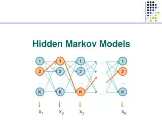
Formal definition of a HHM • A HHM contains the following components: A set of N statesS={S1,S2,…,SN}specify what state a process can be in; a start and an end state can be added to the state set. Transition probability matrixakl specifies how likely the process transits from one state k to another state l. The sequence of states that the process goes through, p=p1p2,…pLis called a path. Thus a path is simply a Markov chain. A set of letters V= {b1,b2,…,bV} that can be emitted in a state. Emission probability matrixek(b) specifies how likely a letter b is emitted in a state k. The sequence of letters emitted, x=x1x2,…xLis called an observation sequence. • Usually, the observation sequence is observable, but the path is not; that is the reason we call the model a hidden Markov model. • Formally we define a HHM as, M={S, V,akl, el(b)}, where,
Example 1: the occasionally dishonest casino • A casino alternates between a fair and a loaded die, the process can be modeled by a four-state HHM. B 0.5 0.5 0.9 0.95 1: 1/6 2: 1/6 3: 1/6 4: 1/6 5: 1/6 6: 1/6 1: 1/10 2: 1/10 3: 1/10 4: 1/10 5: 1/10 6: 1/2 0.045 Fair Loaded 0.095 0.005 0.005 E • In this case, we see the outcome of each roll of a die. If they play L times, we will see a sequence of L symbols (observation sequence), x=x1x2,…xL, but we do not know which die has been used in each roll, i.e., the sequence of dices being used (the path of states), p=p1p2,…pL is hidden from us.
Example 2: prediction of TM helices and loops • The alternation between TM helices and loops in a protein sequence can be also modeled by a two/four-state HHM. • Here, we know the protein sequences (the output of model) x=x1x2,…xL, but we do not know which state generates each of the residues. If we can decode the path p=p1p2,…pL that generates the sequence, we can predict the locations of TM helices and loops.