Chapter 9 One and Two Sample Estimation

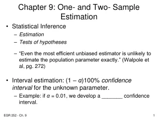
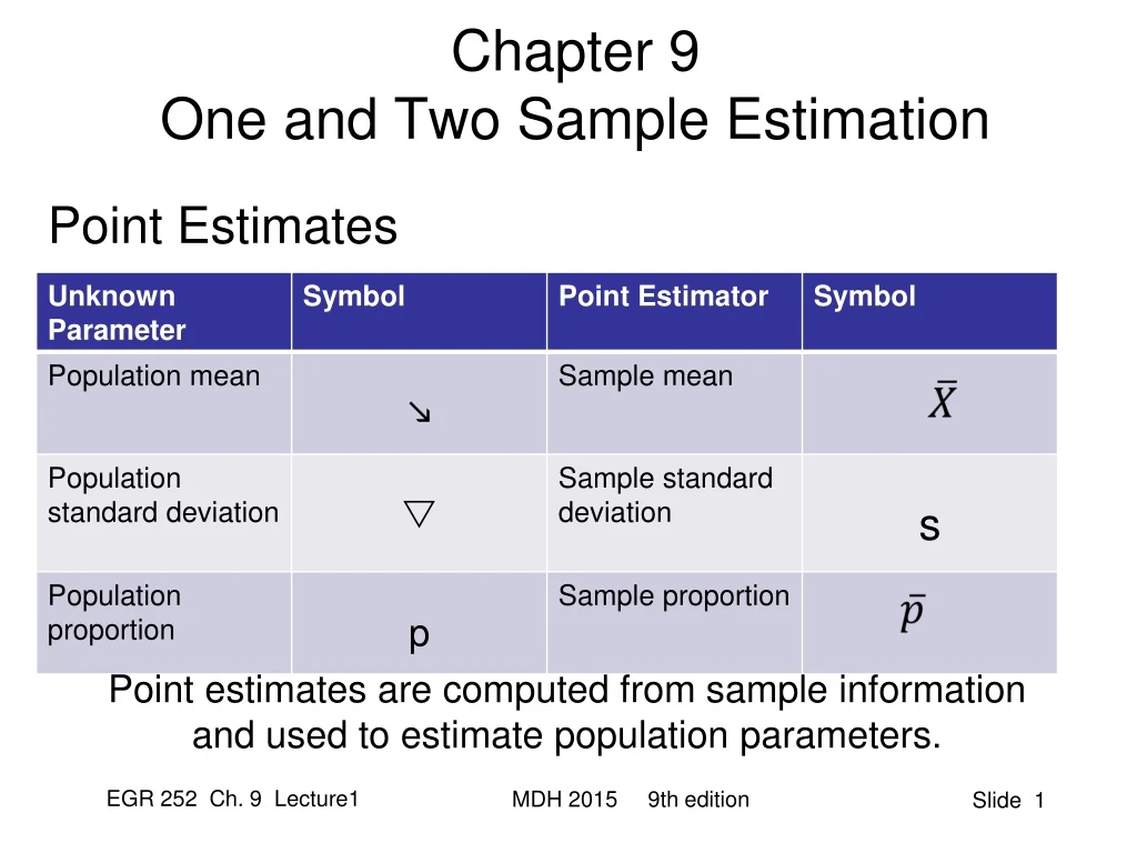
1. Chapter 9One and Two Sample Estimation Point Estimates Point estimates are computed from sample information and used to estimate population parameters. MDH 2015 9th edition

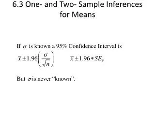
2. Interval Estimation • Interval estimation: The interval in which you would expect to find the value of a parameter. • By taking a random sample, we can compute an interval with upper and lower limits called a (1-a) 100% confidence interval for the unknown parameter • In most a cases the parameter for intervals to be created will be m MDH 2015 9th edition

3. Confidence Intervals MDH 2015 9th edition

4. Confidence Intervals • (1 – α) 100% confidence interval for the unknown parameter. • Example: if α = 0.01, we develop a 99% confidence interval. • Example: if α = 0.05, we develop a 95% confidence interval. MDH 2015 9th edition

5. Single Sample: Estimating the Mean • Given: • σ is known and X is the mean of a random sample of size n, • Then, • the (1 – α)100% confidence interval for μ is Values obtained from Z-table 1 - a a/2 a/2 MDH 2015 9th edition

6. Example A traffic engineer is concerned about the delays at an intersection near a local school. The intersection is equipped with a fully actuated (“demand”) traffic light and there have been complaints that traffic on the main street is subject to unacceptable delays. To develop a benchmark, the traffic engineer randomly samples 25 stop times (in seconds) on a weekend day. The average of these times is found to be 13.2 seconds, and the variance is known to be 4 seconds2. Based on this data, what is the 95% confidence interval (C.I.) around the mean stop time during a weekend day? MDH 2015 9th edition

7. Example (cont.) X = ______________ σ = _______________ α = ________________ α/2 = _____________ Z0.025 = _____________ Z0.975 = ____________ Enter values into equation MDH 2015 9th edition

8. Example (cont.) X = ______13.2________ σ = _____2________ α = ______0.05________ α/2 = __0.025_______ Z0.025 = ___-1.96______ Z0.975 = ____1.96____ Solution: 12.416 < μSTOP TIME < 13.984 Z0.025 = -1.96 Z0.975 = 1.96 13.2-(1.96)(2/sqrt(25)) = 12.416 13.2+(1.96)(2/sqrt(25)) = 13.984 MDH 2015 9th edition

9. Your turn … • What is the 90% C.I.? What does it mean? 90% 5% 5% Z(.05) = + 1.645 All other values remain the same. The 90 % CI for μ = (12.542,13.858) Note that the 95% CI is wider than the 90% CI. MDH 2015 9th edition

10. What if σ2is unknown? • For example, what if the traffic engineer doesn’t know the variance of this population? • If n is sufficiently large (n > 30), then the large sample confidence intervalis calculated by using the sample standard deviation in place of sigma: • If σ2is unknown and n is not “large”, we must use the t-statistic. MDH 2015 9th edition

11. Single Sample: Estimating the Mean(σ unknown, n not large) • Given: • σ is unknown and X is the mean of a random sample of size n (where n is not large), • Then, • the (1 – α)100% confidence interval for μ is: Values obtained from t-table 1 - a a/2 a/2 MDH 2015 9th edition

12. Recall Our Example A traffic engineer is concerned about the delays at an intersection near a local school. The intersection is equipped with a fully actuated (“demand”) traffic light and there have been complaints that traffic on the main street is subject to unacceptable delays. To develop a benchmark, the traffic engineer randomly samples 25 stop times (in seconds) on a weekend day. The average of these times is found to be 13.2 seconds, and the sample variance, s2, is found to be 4 seconds2. Based on this data, what is the 95% confidence interval (C.I.) around the mean stop time during a weekend day? MDH 2015 9th edition

13. Small Sample Example (cont.) n = _______ v = _______ X = ______ s = _______ α = _______ α/2 = ____ t0.025,24 = _______ Find interval using equation below MDH 2015 9th edition

14. Small Sample Example (cont.) n = __25___ v = _24___ X = __13.2_ s = __2__ α = __0.05___ α/2 = 0.025_ t0.025,24 = _2.064_ __12.374_____ < μ < ___14.026____ 13.2 - (2.064)(2/sqrt(25)) = 13.374 13.2 + (2.064)(2/sqrt(25)) = 14.026 MDH 2015 9th edition

15. Your turn A thermodynamics professor gave a physics pretest to a random sample of 15 students who enrolled in his course at a large state university. The sample mean was found to be 59.81 and the sample standard deviation was 4.94. Find a 99% confidence interval for the mean on this pretest. MDH 2015 9th edition

16. Solution X = ______________ s = _______________ α = ________________ α/2 = _____________ (draw the picture) t___ , ____ = _____________ __________________ < μ < ___________________ X = 59.81 s = 4.94 α = .01 α/2 = .005 t (.005,14) = 2.977 Lower Bound 59.81 - (2.977)(4.94/sqrt(15)) = 56.01 Upper Bound 59.81 + (2.977)(4.94/sqrt(15)) = 63.61 MDH 2015 9th edition

17. Standard Error of a Point Estimate • Case 1: σ known • The standard deviation, or standard error of X is • Case 2: σ unknown, sampling from a normal distribution • The standard deviation, or (usually) estimated standard error of X is MDH 2015 9th edition

18. Prediction Intervals • Used to predict the possible value of a future observation • Example: In quality control, an experimenter may need to use the observed data to predict a new observation. MDH 2015 9th edition

19. 9.6: Prediction Interval • For a normal distribution of unknown mean μ, and standard deviation σ, a 100(1-α)% prediction interval of a future observation, x0is if σ is known, and if σ is unknown MDH 2015 9th edition

20. Tolerance Limits (Intervals) • What if you want to be 95% sure that the interval contains 95% of the values? Or 90% sure that the interval contains 99% of the values?  • These questions are answered by a tolerance interval. To compute, or understand, a tolerance interval you have to specify two different percentages. One expresses how sure you want to be, and the other expresses what fraction of the values the interval will contain. MDH 2015 9th edition

21. 9.7: Tolerance Limits • For a normal distribution of unknown mean μ, and unknown standard deviation σ, tolerance limits are given by x + ks where k is determined so that one can assert with 100(1-γ)% confidence that the given limits contain at least the proportion 1-α of the measurements. • Table A.7 (page 745) gives values of k for (1-α) = 0.9, 0.95, or 0.99 and γ = 0.05 or 0.01 for selected values of n. MDH 2015 9th edition

22. Tolerance Limits • How to determine 100(1-γ)% and 1-α. For a sample size of 8, find the tolerance interval that gives two-sided 95% bounds on 90% of the distribution or population. X is 15.6 and s is 1.4 From table on pg. 745, find the corresponding value: n = 8, g = .05, a = 0.1 corresponding k…k = 3.136 x +ks = 15.6 + (3.136)(1.4) Tolerance interval 19.99 – 11.21 We are 95% confident that 90% of the population falls within the limits of 11.21 and 19.99 1-g (boundary or the limits) 1-a (proportion of the distribution) MDH 2015 9th edition

23. Case Study 9.1c (Page 281) • Find the 99% tolerance limits that will contain 95% of the metal pieces produced by the machine, given a sample mean diameter of 1.0056 cm and a sample standard deviation of 0.0246. • Table A.7 (page 745) • (1 - α ) = 0.95 • (1 – Ƴ ) = 0.99 • n = 9 • k = 4.550 • x ± ks = 1.0056 ± (4.550) (0.0246) • We can assert with 99% confidence that the tolerance interval from 0.894 to 1.117 cm will contain 95% of the metal pieces produced by the machine. MDH 2015 9th edition

24. Summary MDH 2015 9th edition