Exploring String Matching Algorithms in Information Retrieval Systems
Learn about classic string matching problems, Brute-Force Algorithm, KMP Algorithm, Boyer-Moore Algorithm, and Suffix Trees for efficient text search and matching. Detailed examples and analysis provided.

Exploring String Matching Algorithms in Information Retrieval Systems
E N D
Presentation Transcript
String Matching Problem • A classical and important problem • Searching engines (like Goole and Openfind) • Database (GenBank) 3 -
Two Phases http://www-igm.univ-mlv.fr/~lecroq/string/ 3 -
Two Phases • Phase 1:generate an array to indicate the moving direction. • Phase 2:make use of the array to move and match string 3 -
An Example for the K.M.P. Algorithm Phase 2 Phase 1 3 -
An Example for the Boyer-Moore Algorithm Phase 2 Phase 1 3 -
The K.M.P. Algorithm • Proposed by Knuth, Morris and Pratt in 1977. • Three cases to illustrate their idea. 3 -
The KMP Alogrithm a a 3 -
j-1 j f(j)=f(j-1)+1 f(j-1) j-1 j a f(j-1) f(j)=f(f((j-1))+1 f(f(j-1)) Phase 1:To Compute the Prefix Function J=k+1 or ? J-k j-1 f(j-1)=k 3 -
j-1 j k=1 f(j)=f(j-1)+1 f(j-1) j-1 j a f(j-1) k=2 f(j)=f(f((j-1))+1 f(f(j-1)) The Prefix Function 3 -
An Example for the K.M.P. Algorithm Phase 2 f(4-1)+1= f(3)+1=0+1=1 Phase 1 f(12)+1= 4+1=5 3 -
The analysis of the K.M.P. Algorithm • O(m+n) • O(m) for computing function f • O(n) for searching P 3 -
An Example for the Boyer-Moore Algorithm Phase 2 Phase 1 3 -
The Rule of Moving the Window • Bad Character Rule • Good Suffix Rule • Good Suffix Rule 1 • Good Suffix Rule 2 3 -
Two Function for the Good Suffix RuleFunction B and G (b) 3 -
Function g1(j) g1(j) 3 -
Functions g2(j) g2(j) 3 -
The Suffix Function f’ f’(j) = k or ? f’(j+1)=k+1 ? 3 -
Function f’ 3 -
Functions f’ and G • Function G can be determined by scanning P twice. • The first one is a right-to-left scan. • The second one is a left-to-right scan. • Function f’ is generated in the first right-to-left scan and some values of G can be determined in this scan. 3 -
The Computation of g1(j) t=f’(j)-1 j 0 0 0 0 0 0 0 0 0 0->3=G(f’(j)-1)=G(7 )=m- g1(j )=m-( m-t+j )=t-j 3 -
The Computation of g2(j=1)(1) m-f’(1)+2 ? j t=f’(j)-1 j 0->8=G(j)=m- g2(j) =m- g2 (1) =m-( m-f’(1)+2) =f’(1)-2=10 - 2 3 -
The Computation of g2(j)(2) m-f’(1)+2 ? j t=f’(j)-2 j 0->11=G(j)=m- g2(j) =m- g2 (j) =m-( m-f’(j)+1) =f’(j)-1=12 -1 3 -
Star Position s 3 -
The Analysis of the Boyer-Moore Algorithm • Phase 1 is O(m) + O(m+||)= O(m+||) • O(m) for G • O(m+||) for computing B • Phase 2 is O((n-m+1)m) • O(m) ,When P is not in T • O(mn) ,When P is in T • the Boyer-Moore-like Algorithms have O(m) • It is more efficient in practice then KMP algorithm. 3 -
The Suffix • S = ATCACATCATCA • The substrings which start with A. • The substrings which start with C. • The substrings which start with T. • Any substrings which starts with A must be one of the following suffixes: S(1), S(4), S(6), S(9) and S(12) 3 -
The Suffix Tree • Each tree edge is labeled by a substring of S. • Each internal node has at least 2 children. • Each S(i) has its corresponding labeled path from root to a leaf, for 1<i<n . • There are n leaves. • No Edges branching out from the same internal node can start with the same character. 3 -