
2.2 Image Compression
E N D
Presentation Transcript
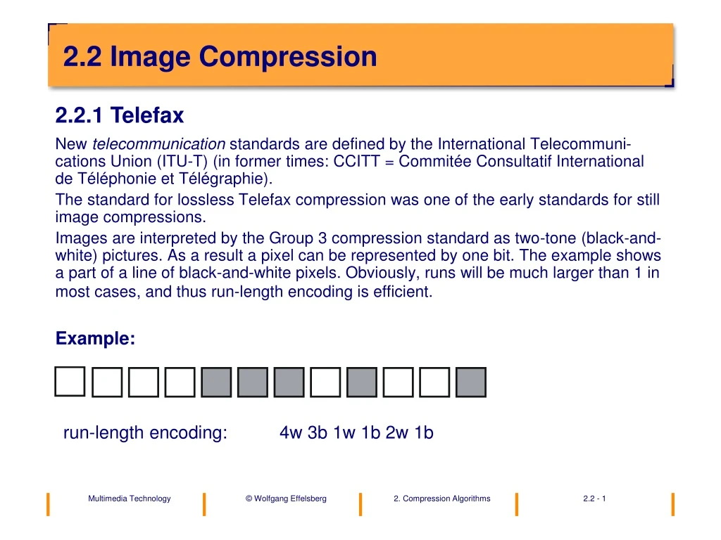
2.2 Image Compression • New telecommunication standards are defined by the International Telecommuni-cations Union (ITU-T) (in former times: CCITT = Commitée Consultatif International de Téléphonie et Télégraphie). • The standard for lossless Telefax compression was one of the early standards for still image compressions. • Images are interpreted by the Group 3 compression standard as two-tone (black-and-white) pictures. As a result a pixel can be represented by one bit. The example shows a part of a line of black-and-white pixels. Obviously, runs will be much larger than 1 in most cases, and thus run-length encoding is efficient. • Example: 2.2.1 Telefax run-length encoding: 4w 3b 1w 1b 2w 1b
Fax Standards of ITU-T • Standard T.4 • First passed in 1980, revised in 1984 and 1988 (Fax Group 3) for error-prone lines, especially telephone lines. • Two-tone (black-and-white) images of size A4 (similar to US letter size) • Resolution: 100 dots per inch (dpi) or 3,85 lines/mm vertical, 1728 samples per line • Objective • Transmission at 4800 bits/s over the telephone line (one A4 page per minute) • Standard T.6 • First passed in 1984 (Fax Group 4) for error-free lines or digital storage.
Compression Standards for Telefax (1) • Telefax Group 3, ITU-T Recommendation T.4 • First approach: Modified Huffman Code (MH) • Every image is interpreted as consisting of lines of pixels. • For every line the run-length encoding is calculated. • The values of the run-length encoding are Huffman-coded with a standard table. • Black and white runs are encoded using different Huffman codes because the run length distributions are quite different. • For error detection, an EOL (end-of-line) code is inserted at the end of every line. This enables re-synchronization in case of bit transmission errors.
Compression Standards for Telefax (2) • Second approach: Modified Read (MR) Code • The pixel values of the previous line are used to predict the values of the current line. • Then run-length encoding and a static Huffman code are used (same as for MH). • The EOL code is also used. • The MH and MR coding alternates in order to avoid error propagation beyond the next line.
2.2.2 Block Truncation Coding (BTC) • This simple coding algorithm is used in the compression of monochrome images. Every pixel is represented by a grey value between 0 (black) and 255 (white). • The BTC Algorithm • Decompose the image into blocks of size n x m pixels. • For each block, calculate the mean value and the standard deviation as • follows: where Yi,j is the brightness of the pixel. 3. Calculate a bit array B of size n x m as follows:
The BTC Algorithm (continued)) • Calculate two grey scale values for the darker and the brighter pixels: • p is the number of pixels having a larger brightness than the mean value of the block, q is the number of pixels having a smaller brightness. • Output: (bit matrix, a, b) for every block.
Decompression for BTC • For every block the gray value of each pixel is calculated as follows: • Compression rate example • Block size : 4 x 4 • Original (grey values) 1 byte per pixel • Encoded representation: bit matrix with 16 bits + 2 x 8 bits for a and b • => reduction from 16 bytes to 4 bytes, i.e., the compression rate is 4:1.
2.2.3 A Brief IntroductiontoTransformations • Motivation forTransformations • Improvement of the compression ratio while maintaining a good image quality. • What is a transformation? • Mathematically: a change of the base of the representation • Informally: representation of the same data in a different way. • Motivation for the use of transformations in compression algorithms: In the frequency domain, leaving out details is often less disturbing to the human visual (or auditive) system than leaving out details in the ori-ginaldomain.
The Frequency Domain • In the frequency domain the signal (one-dimensional or two-dimensional) is represented as an overlay of base frequencies. The coefficients of the fre-quencies specify the amplitudes with which the frequencies occur in the signal.
The Fourier Transform • The Fourier transform of a function f is defined as follows: • where e can be written as • Note: • The sin part makes the function complex. If we only use the cos part the transform remains real-valued.
OverlayingtheFrequencies • A transform asks how the amplitude for each base frequency must be cho-sen such that the overlay (sum) best approximates the original function. • The output signal (c) is represented as a sum of the two sine waves (a) and (b).
One-Dimensional Cosine Transform • The DiscreteCosine Transform (DCT) isdefinedasfollows: with
Examplefor a 1D Approximation (1) • The following one-dimensional signal is to be approximated by the coefficients of a 1D–DCT with eight base frequencies.
Examplefor a 1D Approximation (2) • Some of the DCT kernels used in the approximation.
Example for a 1D Approximation (3) DC coefficient
Example for a 1D Approximation (4) • DC coefficient + first AC coefficient
Example for a 1D Approximation (5) DC coefficient + AC coefficients 1-3
Example for a 1D Approximation (6) • DC coefficient + AC coefficients 1-7
2.2.4 JPEG • The Joint Photographic Experts Group (JPEG, a working group of ISO) has developed a very efficient compression algorithm for still images which is commonly referred to with the name of the group. • JPEG compression is done in four steps: • 1. Image preparation • 2. Discrete Cosine Transform (DCT) • 3. Quantization • 4. Entropy Encoding
Color Models • The classical color model for the computer is the RGB model. The color value of a pixel is the sum of the intensities of the color components red, green and blue. The maximum intensity of all three components results in a white pixel. • In the YUV model, Y represents the value of the luminance (brightness) of the pixel, U and V are two orthogonal color vectors. • The color value of a pixel can be easily converted from model to model. RGB Model YUV Model An advantage of the YUV model is that the value of the luminance is directly avail-able. That implies that a grey-scale version of the image can be created very easily. Another point is that the compression of the luminance component can be different from the compression of the chrominance components.
Color Subsampling • One advantage of the YUV color model is that the color components U and V of a pixel can be represented with a lower resolution than the luminance value Y. The human eye is more sensitive to brightness than to variations in chrominance. There-fore JPEG uses color subsampling: for each group of four luminance values, one chrominance value for U and one for V is sampled. In JPEG, four Y blocks of size of 8x8 together with one U block and one V block of size 8x8 each are called a macroblock.
JPEG "Baseline" Mode • JPEG Baseline Mode is a compression algorithm based on a DCT transform from the time domain into the frequency domain. • Image transformation • FDCT (Forward Discrete Cosine Transform). Very similar to the Fourier transform. It is used separately for every 8x8 pixel block of the image. with This transform is computed 64 times per block. The result are 64 coefficients in the frequency domain.
Base “Frequencies” for the 2D-DCT To cover an entire block of size of 8x8 we use 64 base “frequencies”, as shown below.
Example of a Base Frequency The figure below shows the DCT kernel corresponding to the base frequency (0,2) shown in the highlighted frame (first row, third column) on the previous page.
Example: Encoding of an Image with the 2D-DCT DCT block size: 8 x 8 original one coefficient four coefficients 16 coefficients
upper limit a/2 quantization interval a of size a a/2 lower limit Quantization: Basics • The next step in JPEG is the quantization of the DCT coefficients. Quantiz-ation means that the range of allowable values is subdivided into intervals of fixed size. The larger the intervals are chosen, the larger the quantization error will be when the signal is decompressed. Maximum quantization error: a/2
Quantization: Quality vs. Compression Ratio Coarse Quantization Fine Quantization .. .. 100 ........... Range of Values 011 010 001 00100 00011 00010 000 00001 00000
Quantization Table • In JPEG the number of quantization intervals can be chosen separately for each DCT coefficient (Q-factor). The Q-factors are specified in a quantiz-ation table. • Entropy-Encoding • The quantization step is followed by an entropy encoding (lossless en-coding) of the quantized values: • The DC coefficient is the most important one (basic color of the block). The DC coefficient is encoded as the difference between the current DC coefficient value and the one from the previous block (differential co-ding). • The AC coefficients are processed in zig-zag order. This places coeffici-ents with similar values in sequence.
Quantization and Entropy Encoding • Zig-zag reordering of the coefficients is better than a read out line-by-line because the input to the entropy encoder will have a few non-zero and many zero coefficients (representing higher frequencies, i.e., sharp edges). The non-zero coefficients tend to occur in the upper left-hand corner of the block, the zero coefficients in the lower right-hand corner. • Run-length encoding is used to encode the values of the AC coefficients. The zig-zag read out maximizes the run-lengths. The run-length values are then Huffman-encoded (this is similar to the telefax compression algorithm).
Quantization Factor and Image Quality • Example: Palace in Mannheim • Palace, original imagePalace image with Q=6
Palace Example (continued) • Palace image with Q=12 Palace image with Q=20
Flower Example (1) • Flower, original image Flower with Q=6
Flower Example (2) • Flower with Q=12 Flower with Q=20
2.2.5 Compression with Wavelets • Motivation • Signal analysis and signal compression. • Known: image compression algorithms • based on the pixel values (BTC, CCC, XCCC) • based on a transformation into the frequency domain, such as Fourier • Transform or DCT
Examples • “Standard” representation of a signal: • Audio signal with frequencies over time • Image as pixel values on places of the screen
The Frequency Domain • In the frequency domainthe changes of a signal are our focus. • How strong is the variation of the amplitude of the audio signal? • How strong deviates one pixel from the previous? • Which frequencies are contained in the given signal?
Time-to-Frequency Transformations • A transformation weights every single frequency to prepare it for an accumulation of all frequencies for to reconstruction of the original signal. • The output signal (c) consists of the sum of the two sine waves (a) und (b).
Problems with the Fourier Transformation • If we look at a signal with a high “locality”, a great manysine and cosine oscillations must be added. The example shows a signal (upper figure), which disappears on the edges. It is put together with sine oscillations from 0-5 Hz and 15-19 Hz (lower figure). • Wanted: A frequency representation based on functions that feature a high locality, i.e., are NOT periodic. • The solution: Wavelets
What is a Wavelet ? • A wavelet is a function that satisfies the following permissibility condition: • As follows: • A wavelet is a function that exists only in a limited interval.
Example Wavelets • Haar Wavelet • Mexican Hat • Daubechies-2 1 0 0 1/2 1 -1
Application of Wavelets • We limit the further discussion to • Discrete Wavelet Transformations (DWTs) • dyadic DWTs (i.e., those based on a factor of 2) • orthogonal wavelets. • StéphaneMallat discovered a very interesting correlation between orthogonal wavelets and filters which are much used in signal processing today. That is the reason for the terms “high-pass filter” (~ wavelet) and “low-pass filter” (~ scaling function) which we will use in the following.
Amplitude 4 3 2 Signal 1 Time Example: Haar Transformation (1) • We perform a wavelet transformation with the Haar wavelet without caring too much about the theory. • Objective: Decomposition of a one-dimensional signal (e.g., audio) in the form of wavelet coefficients. 1 2 2 3 2 3 4 1 1 2 2 1 1
Example: Haar Transformation (2) • How can we represent the signal in another way without any loss of infor-mation? A rougher representation uses the mean value between two values. • Filter for the calculation of the mean value (approximation): A filter is placed over the signal. The values, which lay “one upon the other”, are multiplied and all together added ( convolution). Amplitude 4 3 Approximation 2 Signal 1 Time 1 2 2 3 2 3 4 1 1 2 2 1 1 Signal 1.5 2.5 2.5 2.5 1.5 1.5 Approximation 1/2 1/2
Example: Haar Transformation (3) • With the representation of the signal by the approximation we loose information! To reconstruct the signal we must know how far the two values are away from the mean value. • Filter for the calculation of the differences (detail): Amplitude 4 3 Mean value 2 Signal 1 Detail Time 1 2 2 3 2 3 4 1 1 2 2 1 1 Signal 1.5 2.5 2.5 2.5 1.5 1.5 Mean value -0.5 -0.5 -0.5 1.5 -0.5 0.5 Detail 1/2 -1/2
1 2 2 3 2 3 4 1 1 2 2 1 1 Signal 1.5 2.5 2.5 2.5 1.5 1.5 Mean value -0.5 -0.5 -0.5 1.5 -0.5 0.5 Detail Example: Haar Transformation (4) • We have transformed the original signal into another representation. Notice: The number of coeffi-cients we need for a complete representation is unchanged. (that corresponds to the meaning of the mathematical term “base transformation”). • To reconstruct the original signal with the approximation and the details synthesisfiltersareused. • With that: • 1.5*1+(-0.5)*1 = 1 (synthesis of the first value) • 1.5*1+(-0.5)*(-1) = 2 (synthesis of the second value) • 2.5*1+(-0.5)*1 = 2 (synthesis of the first value) • 2.5*1+(-0.5)*(-1) = 3 (synthesis of the second value) • etc. 1 1 Synthesis filter for the first value 1 -1 Synthesis filter for the second value
1/2 1/2 1/2 -1/2 1 1 1 -1 Example: Haar Transformation (5) • All together we need four filters for the decomposition and the synthesis of the origi-nal signal: • Approximation filter for the mean value • Detail filter for the differences • Synthesis filter for the first value • Synthesis filter for the second value • The decomposition of the signal into approximations and details can now be conti-nued with the input signal. • Declarations: • Approximation filter := low-pass filter • Detail filter := high-pass filter
High- and Low-Pass Filters • The Figure shows a low-pass filter. A low-pass filter lets lower frequencies pass (multiplication with 1) and blocks out higher frequencies (multiplication with 0). In real filter implementations the edge is not sharp. • A high-pass filter works vice-versa.