Download
1 / 42
420 likes | 576 Vues
Emissions & Air Quality Modeling for Regional Haze Planning in the WRAP Region. John Vimont National Park Service/WRAP Modeling Forum Co-Chair Reasonable Progress/SO x /NO x Workshop Tucson, AZ – January 10, 2006. Regional Modeling Center – 2006 Simulations.

E N D
Emissions & Air Quality Modeling for Regional Haze Planning in the WRAP Region John Vimont National Park Service/WRAP Modeling Forum Co-Chair Reasonable Progress/SOx/NOx Workshop Tucson, AZ – January 10, 2006
Regional Modeling Center – 2006 Simulations Modeling – 3 tracks for 2006, emphasis changing to planning/control strategies • 2002 Actual emissions/air quality modeling – “base02a,b,c…” series – will not be shown today • Used for model performance evaluation, required by EPA • 2000-04 Regional Haze Baseline Period emissions/air quality modeling – “planning02a,b…” series • Used for comparison to baseline monitoring data and projecting 2018 visibility • 2018 Projection emissions/air quality modeling – “base18a,b,c…” series • Series starts as “base case” – will evolve into “regional control strategy runs” to support the various SIPs • Includes source apportionment, sensitivity runs
Emissions changes 2002 Actual Case to 2000-04 Planning Case (“base02a” to “planning02a”) • Emissions changes from “base02a” to “planning02a” • Area – updates/corrections, mostly in California • Actual 2002 replaced with 2000-04 “average, representative” data for all WRAP fire categories • Oil & gas – updates/corrections, mostly in California • Nonroad mobile – updates/corrections, mostly in California, also CO & MT • On-road mobile – updates/corrections, mostly in California, also CO & MT • Commercial marine shipping – changes/corrections entire West Coast • Road dust – updates/corrections, mostly in California • Fugitive dust – updates/corrections, mostly in California • Point – updates/corrections, several different states • Begin using 2000-03 average monthly temporal emissions profiles for EGUs, by state and fuel type • All other emissions are the same between”base02a” and “planning02a”
“Planning02a” Emissions Modeling QA Based on the known inventory differences (between base02a and plan02a) and the QA difference plots: 1) Area - Known changes: Revised CA EI, Revised WA, ND, OR, & UT EIs, Revised Mexico99, VISTAS baseF (non-fire sources only) • Seeing inventory differences in all of the WRAP states except OR. Some changes in Canada PM due to an expansion of the list of dust sources that we extracted from this inventory relative to b02a. Otherwise, all of the changes that we expect to see are in the correct locations. Also changes in CO due to the Broomfield County correction. • The inventory comparison between b02a and plan02a show that the changes occurred where expected. The spatial plots show differences in other areas of the domain due to temporal profiles updates. 2) WRAP Fires - Known changes: 2000-04 “typical, representative” WRAP fire EIs replace actual 2002 fire EIs • Confirmed that RMC used different inventories for the b02a and plan02a simulation, actual for the former (deliver date 07/06/05) and typical for the latter (deliver dates: non-fed rangeland 04/05/05, ag 07/01/05, wf 10/21/05, wild fire use 10/21/05, anth rx 10/21/05, nat rx 10/21/05). 3) Fugitive Dust - Known changes: Revised CA EI, Revised WA,ND,OR,UT EI, Revised Mexico99, VISTAS baseF • Increases in Canada that are related to the expansion of the fugitive dust list. Changes outside of the WRAP states that are related to the application of different temporal profiles. In particular the MWRPO and CENRAP show large month-to-month differences that are the result of temporal allocation differences. • Obvious changes in CA; changes to the area EI didn't affect the fugitive dust sources in ND, OR, UT, or WA or the VISTAS states. There are also changes in Mexico, as expected. There are also changes in CO due to the Broomfield County correction. • Inventory comparisons show changes where expected: CA, Mexico, and Canada. All other differences in the spatial plots are due to temporal profile updates. 4) On-Road Mobile - Known changes: Revised CA EI, Revised WRAP (non-CA) EI w/ updates to MT, Revised Mexico99 • There are changes in Mexico, CA, MT, and CO (due to the Broomfield County correction). There are also changes throughout the WRAP states in the winter months due to an error in the Base02a mobile EI. This will be corrected in the next Base02 simulation. • CA and MT differences are seen in the inventory comparisons, as well as the spatial plot differences.
“Planning02a” Emissions Modeling QA, continued 5) Non-Road Mobile - Known changes: Revised CA EI, Revised WRAP region aircraft/locomotive (changes to CA only), Removed CA in-/near-shore shipping (covered in gridded shipping EI), VISTAS baseF, Revised Mexico99 (incl. plane/train/ships/border x from area) • Changes in CA, VISTAS, and Mexico only due to the inventory updates, none in any of the other WRAP states, CANADA, or RPOs; changes throughout the VISTAS, MWRPO, and MANE-VU states due to temporal profiles updates and inventory changes (for VISTAS); small changes in PM in Canada due to temporal profile changes 6) Oil & Gas - Known changes: Revised CA EI (extracted from area) • As expected, differences in CA only. 7) Point - Known changes: Revised CA EI, Revised wrap EI for AK,AZ,MT,NM,OR,UT,WA,WY, Revised WRAP tribal EI, VISTAS typical 2002 baseF, Revised Mexico 1999, Updated typical temporal profiles for EGUs • Changes throughout the domain except for Canada. Can't discern differences between inventory and temporal profile updates. 8) Road Dust - Known changes: Revised CA EI (extracted from area, now an annual EI, no longer seasonal), VISTAS typical 2002 baseF • Only differences in CA and small change in CO due to Broomfield County correction. 9) Commercial Marine - Known changes: Updates to Pacific waters and CA in-/near-shore • No differences in shipping lane emissions; only differences in CA near-shore emissions; no differences in Gulf Conclusions • All the expected changes show up in the Plan02a simulation. Confirmed the inventory changes using the Smkreport outputs. The effects of the temporal profiles updates are seen along with the inventory changes in the spatial difference plots. • Comfortable with the Plan02a emissions in that it looks like all of the data got through as expected.
2000-04 Baseline Period SOx Emissions Density Mapfrom SMOKE from “planning02a”
2000-04 Baseline Period NOx Emissions Density Mapfrom SMOKE from “planning02a”
Emissions changes 2002 Planning Case to 2018 Base Case version 1 (“planning02” to “base18a”) Here's a list of the inventories that have changed between 2002 Planning and 2018 Base v1: • Area Sources- All U.S. inventories projected to 2018, Dust moved to fugitive and road dust sectors • Fugitive Dust - All U.S. inventories projected to 2018 • Road Dust - All U.S. inventories projected to 2018, No MWRPO emissions • On-road mobile- All U.S. inventories projected to 2018 • Non-road mobile- All U.S. inventories projected to 2018 • Ag NH3 - CENRAP and MWRPO projected to 2018, WRAP unchanged • Offshore - Gulf of Mexico emissions projected to 2018, U.S. West Coast unchanged • Point - All U.S. inventories projected to 2018, Several updates for typical EGU temporal profiles • WRAP Oil & Gas - Projected to 2018
2018 Base Case (“base18a”) Emissions Modeling QA Based on the known inventory differences between plan02a and base18a & the QA difference plots: 1) Area - Known changes: All U.S. inventories projected to 2018; Dust moved to fugitive and road dust sectors; same list of dust sources as plan02a • Confirmed consistent inventory categories and the same ancillary data for each simulation. All of the changes that we're seeing in the spatial plots appear to be correlated with the inventory changes, some pollutants went up, some went down and the spatial plots are consistent with these changes. No changes in Canada or Mexico, as expected. • Trends that are worth looking into: • CA area NH3 emissions are 1/2 of the 2002 value in 2018. • Iowa area NH3 emissions are double in 2018 but the changes only appear to happen in a few grid cells on the eastern part of the state. • MO area NH3 emissions are up 70% in 2018. • NM area SO2 emissions are up over 200% in 2018 2) Fugitive Dust - Known changes: All U.S. inventories projected to 2018 • Confirmed consistent inventory categories and the same ancillary data for each simulation; Pace transport factors applied to inventories. The inventory changes are consistent with the patterns in the spatial plots. NV is the only state that shows a net decrease in emissions in 2018, everywhere else shows net increases. • Utah is the largest change in the WRAP region, it shows increases in PM2.5 and PMC of 57% and 86%, respectively. The interesting thing about this is that it appears to be concentrated in only a couple of grid cells around the Great Salt Lake. • Trends: • The big red increases in IL and IN are correlated with inventory increases of around 50% for each state. These percentage increases are significant between these two states are 2nd and 5th largest sources of PMC from fug dust in the country. • AZ shows around 50% increase for all PM pollutants, this is net, between the spatial plots show some areas of decrease 3) Road Dust - Known changes: All U.S. inventories projected to 2018; No MWRPO emissions • Confirmed consistent inventory categories and the same ancillary data for each simulation; Pace transport factors applied to inventories. No differences in Mexico or Canada; mostly increases through the U.S. There are not spatial plots yet, but from the inventory summaries here are some trends: • Trends: • NV has the largest increase in PMC in the U.S. at +53% • ME has the largest decrease in PMC in the U.S. at -16% • ND is the only WRAP state that decreases in PMC at -4.3%
2018 Base Case (“base18a”) Emissions Modeling QA, continued 4) On-road mobile - Known changes: All U.S. inventories projected to 2018 • Confirmed consistent inventory categories and the same ancillary data for each simulation. I've only checked the inventory values for the WRAP states against the spatial difference plots. The inventory differences support the trends in the spatial plots. One discrepancy is with ND, the inventory differences indicate that it is towards the top of changes for most pollutants (+56% CO, +80% NOx, +90% SO2), but the spatial diff plots aren't showing it as having large differences. Likely due to the fact that it's base emissions are relatively low to begin with. • Trends: • In the WRAP states CO, NOx, SO2, VOC show across the board decreases; NH3 and PM show across the board increases (except primary sulfate, except for CA it shows decreases, CA shows an increase). 5) Non-road mobile- Known changes: All U.S. inventories projected to 2018 • Commercial marine inshore shipping emissions (port activities) for OR and WA were missed for Base18a, this needs to be added in the future 2018 runs. There are a number of other changes that need to be checked: CENRAP switched from a monthly to annual inventory from Plan02a to Base18a. MWRPO provided annual planes/trains/ships for 2018, they didn't have this for plan02a. 6) Ag NH3 - Known changes: CENRAP and MWRPO projected to 2018 7) Offshore - Known changes: Gulf of Mexico emissions projected to 2018 8) Point - Known changes: All U.S. inventories projected to 2018. Several updates for EGU temporal profiles • Confirmed consistent inventory categories and the same ancillary data for each simulation. There are no spatial plots yet, but here are the trends I'm seeing in the inventory comparisons. No differences in Canada or Mexico. Differences throughout the US and Tribal lands of varying degree. Here's a few that stand out: • Trends: • 42,962% increase in NH3 for Arkansas (started at 1 tpy in 2002, up to 456 in 2018) • MWRPO sources showing some very large increases in NH3 and PM (>100%) going to 2018. • CA NH3 decreases by 100% • The changes are pretty much all over the place for US point sources, mostly decreases in SO2, but some notable increases, such as a 120% increase in Michigan, an 80% increase in Wisconsin, 17.5% increase in California. Big decreases in point SO2 included many large changes in the MANE-VU states (-84.4% in NH and -72.8% in MA) and the biggest change in the WRAP is 52.6% decrease in NV. 9) WRAP Oil & Gas - Known changes: Projected to 2018
2018 Base Case (“base18a”) Emissions Modeling QA, continued Status check a few days into “base18a” CMAQ run: • Found and corrected a problem in the processing of the 2018 locomotive emissions • The 2018 CMAQ run is showing large sulfate increases in the Chicago area, should we expect this because of changes in the MWRPO 2018 data? • In the 2018 on-road we have small increases in PSO4, PMC and POA but we have reductions in NO, CO and other species. Any idea why PSO4 would increase in the 2018 California on-road? Emissions QA Conclusions • Generally comfortable with EI data changed from “planning02” • Need to update/correct port activity emissions data for OR and WA • Need to address for subsequent 2018 simulations (base18b, et cetera): • Emissions and AQ changes outside the WRAP region • Review unusual emissions changes in WRAP region, e.g., 100% decrease in California point source NH3 emissions
SOx Emissions Density Change Map from SMOKEfrom “planning02a” to“base18a”
NOx Emissions Density Change Map from SMOKEfrom “planning02a” to“base18a”
Model Challenges • Meteorology • Resolution • Clouds • Emissions • Point, area, mobile pretty good • Fire, dust, ammonia more uncertain • Depend on meteorology • Dispersion • Resolution
More Model Challenges • Chemistry • Secondary pollutants dependent on many parameters • Nitrate mostly NH4NO3 in model • In equilibrium i.e. HNO3+NH3NH4NO3 • Dependent on Temperature and Relative Humidity • HNO3 & NH3 deposit and are soluble • Measured nitrate may be NaNO3 or CaNO3 • Coarse mode tail • Organics • Unclear how much secondary versus primary • Biogenic versus Anthropogenic • SO4 highly influenced by clouds
SO4 Concentration Change Map from CMAQ Resultsfrom “planning02a” to“base18a”
NO3 Concentration Change Map from CMAQ Resultsfrom “planning02a” to“base18a”
Distance ~ 5 miles [(NH4)2SO4] = 1.14 µg/m3 [NH4NO3] = 0.13 µg/m3 [Organics] = 0.72 µg/m3 [EC] = 0.1 µg/m3 [Soil] = 1.44 µg/m3 [CM] = 6.69 µg/m3 Aerosol bext= 16.4 Mm-1 SVR = 148 km
Individual Sites • SIPs based on individual class I areas • Model performance varies by area • Model performance varies by constituent • Model run for 1 year (2002) • Progress based on 5-year average of 20% worst
Conclusions/Considerations • Modeling is one tool to use in preparing SIPs • Should be used with corroborating information • Examine model’s usefulness site-by-site & constituent-by-constituent • Limited by one year (2002) versus 5-year average for RHR baseline • Overall, base/planning model looks quite reasonable and should prove useful • All will work with the magic of relative reduction factors! Stay tuned…
Next Steps • Resolve current QA questions • Apply further controls (tbd) • Source attribution with CAMx PSAT
We're Professionals Don't Try This At Home