Download
1 / 23
230 likes | 358 Vues
Academy of Economic Studies, Bucharest Doctoral School of Finance and Banking. Long Memory and Structural Breaks in Romanian Inflation Rates. MSc Student: Virgil Savu Supervisor: Professor Moisa Altar. - July 2003 -. Contents:. ■ Memory

E N D
Academy of Economic Studies, Bucharest Doctoral School of Finance and Banking Long Memory and Structural Breaks in Romanian Inflation Rates MSc Student: Virgil Savu Supervisor: Professor Moisa Altar - July 2003 -
Contents: ■ Memory ■ Review ■ Unit root tests ■ Chow test of structural change ■ R/S analysis ■ Spectral analysis ■ GPH ■ Local Whittle ■ Conclusions
Memory Memory is the series property to depend on its own past realizations. From the viewpoint of memory characteristics data generating processes can be classified as follow : ■ Processes with no memory: ■ Processes with infinite memory: - for an AR (1) process a1 is also the first order autocorrelation; - if a1=1 the process is said to contain an unit root (d=1) and the influence of the past shocks to present realisations never decreases; - for a1 =1, the above becomes the random walk model:
Between those two extremes, processes with finite memory can be found: ■ Processes with short memory: • if all the roots of polynomial lie outside the unit circle • then the influence of the shocks decrease exponentially and converge to zero at a • rate depending on the AR coefficients; • - for a1 <1 in the ARMA above and setting y0=0, • the direct exponential decay of the autocorrelation function is the key feature of • short memory processes when it comes to persistence ; ■ Processes with long memory: The model with d=1 corresponds to a model with persistence of shocks. However, persistence need not be infinite so it can be modelled whit d > 0 and < 1. The autoregressive fractionally integrated moving average (ARFIMA) model aims to capture the long memory that is apparent in a time series by allowing the difference parameter to take noninteger values.
A series Xt follows an ARFIMA (p,d,q) process if: where are the AR and MA polynomials. We assume that all the roots of those polynomials lie outside the unit circle. The fractionally differencing term can be written as an infinite order MA process using the binomial expansion: where For an ARFIMA (0,d, 0) applying the expansion to Xt yields: where the autoregressive coefficients are expressed in terms of the gamma function: Hosking 1981 . The process is both stationary and invertible if the roots of the AR and MA polynomials are outside the unit circle and –0.5<d<0. The ARFIMA processes with 0<d<0.5 displays long memory and is stationary. For 0.5<d<1, the process is invertible but nonstationary. For d>1 the process is not mean–reverting, and a shock to the process causes it to deviate away from its starting point.
Review In the ’80 the persistence of inflation was discussed in the I(0)-I(1) alternative aproach: ■ Nelson and Schwert (1977) ■ Barsky (1987) ■ Ball and Cecchetti (1990) ■ Bruner and Hess (1993) The possibility that the order of integration could be between 0 and 1 give rise to an explosion of fractionally integrated models in the ’90. Strictly to inflation, the most important studies are: ■ Hassler and Wolters (1995) ■ Baillie, Chung and Tieslau (1996) ■ Bos, Frances and Ooms (1999) ■ Hsu and Kuan (2000) ■ Caporale and Gil-Alana (2002)
The data used in the dissertation paper is monthly Romanian inflation rates taken from December 1990 trough March 2003, computed from the Consumer Price Index by taking the first difference of the logarithmic transformed series. The raw data is show in the figure below: .28 .24 .20 .16 .12 .08 .04 .00 1992 1994 1996 1998 2000 2002 d L O G ( C P I )
Unit root tests Memory or persistence is closely related to the order of integration. To test for dependence in the context of nonfractionally integration is equivalent to establish whether the series is I(0) or I(1). The commonly used tests are KPSS, ADF and PP. The null of the KPSS test is covariance stationary and is based on the residuals from the OLS regression of on the exogenous variables : The LM statistic is defined as: where S(t) = and is an estimate of the spectral density of the residuals at zero frequency. The optimal lag is selected according to: - Andrews (1991) assumes that the sample follow a AR(1) process: Bartlett kernel • Newey and West (1994) is based on a truncated weighted sum of • the cross-moments: Quadratic Spectral kernel
Null Hypothesis: Y is stationary Bandwidth: 7.96 (Andrews using Quadratic Spectral kernel) Exogenous: Constant LM-Stat. Bandwidth: 9 (Newey-West using Bartlett kernel) Kwiatkowski-Phillips-Schmidt-Shin test statistic Bandwidth: 6.97 (Newey-West using Quadratic Spectral kernel) Bandwidth: 9.12 (Andrews using Bartlett kernel) 0.903873 Asymptotic critical values*: 1% level 0.739000 LM-Stat. LM-Stat. LM-Stat. Kwiatkowski-Phillips-Schmidt-Shin test statistic Kwiatkowski-Phillips-Schmidt-Shin test statistic Kwiatkowski-Phillips-Schmidt-Shin test statistic 5% level 0.463000 0.994218 0.928973 0.922180 Asymptotic critical values*: Asymptotic critical values*: Asymptotic critical values*: 1% level 1% level 1% level 10% level 0.739000 0.739000 0.739000 0.347000 *Kwiatkowski-Phillips-Schmidt-Shin (1992, Table 1) 5% level 5% level 5% level 0.463000 0.463000 0.463000 10% level 10% level 10% level 0.347000 0.347000 0.347000
Null Hypothesis: Y has a unit root Null Hypothesis: Y has a unit root Exogenous: Constant Exogenous: Constant Bandwidth: 5.86 (Newey-West using Quadratic Spectral kernel) Lag Length: 1 (Automatic based on SIC, MAXLAG=13) t-Statistic Adj. t-Stat Prob. Prob. Phillips-Perron test statistic Augmented Dickey-Fuller test statistic -6.267296 -4.470810 0.0000 0.0003 Test critical values: Test critical values: 1% level 1% level -3.475500 -3.475184 5% level 5% level -2.881260 -2.881123 10% level 10% level -2.577291 -2.577365 ADF and PP have the null of containing a unit root and are based on t-ratios. ADF assumes the normality of the errors and when the errors are correlated the t-statistic does not have the asymptotically t-distribution. So, the critical values are based on simulations. The most extensive one is that of MacKinnon (1991). PP correct the t-ratios allowing for a limited degree of serial correlation. The resulting Z-statistics have the asymptotically student distribution.
As noted in Baillie, Chung and Tieslau (1996) the combined use of ADF, PP and KPSS test statistics give rise to four possible outcomes: ■ rejection by the ADF and PP and failure to reject by the KPSS is viewed as strong evidence of covariance stationary I(0) process; ■ failure to reject by the ADF and PP and rejection by the KPSS statistic is strongly indicative of a unit root I(1) process; ■ failure to reject by all ADF, PP and KPSS is probably due to the data being insufficiently informative for the long-run characteristics of the process; ■ rejection by all ADF, PP and KPSS indicates that the process is described by neither I(0) and I(1) processes and that is probable better described by the fractional integrated alternative. All tests reject their null at 1% significance level, so a long memory fractional- integrated alternative is quite appealing for Romanian inflation.
Y=C(1) Chow Breakpoint Test: 1994:12 1997:06 Variable Chow Breakpoint Test: 1993:12 1997:04 Coefficient Std. Error t-Statistic Prob. C F-statistic F-statistic 25.92426 0.043997 Coefficient 34.13225 Std. Error 0.013408 Probability Probability t-Statistic 3.281420 Prob. 0.000000 0.0013 0.000000 AR(1) Log likelihood ratio Log likelihood ratio 0.889058 110.9525 57.09833 0.052922 Probability Probability 16.79931 0.0000 0.000000 0.000000 C(1) 0.050205 0.003954 12.69572 0.0000 MA(1) -0.529560 0.100522 -5.268083 0.0000 R-squared 0.410372 Mean dependent var 0.049801 Adjusted R-squared 0.402183 S.D. dependent var 0.048020 S.E. of regression 0.037128 Akaike info criterion -3.728675 Sum squared resid 0.198506 Schwarz criterion -3.667646 Log likelihood 277.0576 F-statistic 50.11086 Durbin-Watson stat 1.908732 Prob(F-statistic) 0.000000 Chow test of structural change One should be very carefully when testing for long memory if structural breaks occurred. And there are structural breaks in Romanian inflation. To formally test for the existence of the breaks I used the Chow breakpoint test. This test necessitates a model specification and a priori dates for the breaks. I use the test to see where the series experience mean changing and when the best fitted ARMA representation becomes unstable. The exact dates for the breaks are taken where the reported F-statistics and Log likelihood ratios are maximized.
R/S analysis To detect long-range dependence in financial markets, Mandelbrot refined Hurst’s R/S statistic. The R/S statistic is the range of partial sums of deviations of a time series from its mean, rescaled by its standard deviation. Let t = 1,2… where = , and are random variables with mean 0 and Y(t) the partial sum of t observations. Then the rescaled range statistic is: where When the errors are i.i.d. via functional central limit theory it can be shown that: . Lo (1991) showed that when the errors are correlated (strong mixing) the R/S do not have the above limiting distribution so the null of short memory is rejected to often. To allow for a limited degree of serial correlation Lo modified the R/S by letting the denominator to take the form of the “long-run variance”, specifically:
T V(T,0) V(T,q) V(T,10) V(T,20) Kernel 148 3.3663879400 1.5478684650 1.4961427840 1.2311548840 BT 148 3.3213233010 1.5400482670 1.4221796900 1.1572671420 QS T V(T,0) V(T,q) V(T,10) V(T,20) Kernel 148 1.7295304890 1.2863583570 1.2690816140 1.2676390590 BT 148 1.7295304890 1.2662254040 1.2268272460 1.2638703410 QS Critical values for 1%, 5%, 10% are 2.001, 1.747, 1.620 where and are the usual sample variance and autocovariance estimators and: is the Bartlett kernel. In order to choose the optimal truncation lag q the data dependent formula of Andrews (1991) is proposed. Lo showed that when data are short range dependent The Mandelbrot statistic is the coresponding V(T,0). The optimal truncation lag q* is 9 for the Bartlett Kernel and 8 for the quadratic spectral. With no structural change With beaks at 1993: 12 and 1997 :04 The critical values are computed as fractiles of the distribution of the range of a standard Brownian bridge on the unit interval. The cdf is given in Feller (1951):
2.5 2 1.5 1 0.5 0 -0.5 -1 -1.5 -2 -2.5 -2 -1 0 1 2 3 4 5 6 7 8 Spectral analysis In ordinary time series analysis we are mainly focused on serial dependencies (autocorrelations) in the time series. This is usually called “time domain analysis”. In spectral analysis or “frequency domain analysis” we are interested in cyclical regularities of the underlying generating process of the observed time series. Conversion from time domain to frequency domain is done by Fourier transformation. The goal of the analysis is to determine how important cycles of different frequencies are in accounting for the behavior of the series. This is achieved by estimating the spectral density. where is the periodogram function. Periodogram of inflation Spectrum of inflation 60 50 40 30 Power Imaginary axis 20 10 0 0 0.5 1 1.5 2 2.5 3 3.5 Angular frequencies Real axis
GPH The spectral density of a stationary ARFIMA(0,d,0) process , integrated of an order d between –0.5 and 0.5 at 0 frequency has the form: When parameter d is well estimated then is white noise and when the frequency tends to 0, is a good estimate of the spectral density of Y at frequency 0 and we can write: Taking the logarithm results: For a given series the periodogram is given by: For frequencies close to 0 the term tends to zero and the previous equation can be written as an OLS regression equation: If the OLS estimator of d is consistent then the error term is white noise.
c=0.45 c=0.5 c=0.55 c=0.65 c=0.75 m=T/2 With no structural breaks d 1.033037 0.735025 0.595491 0.595058 0.518525 0.491928) t-stat (-3.619196) (-2.915859) (-2.899099) (-3.996341) (-5.179419) (-6.221068) With breaks at 1993 :12 1997 :04 d 0.457745 0.337626 0.26537 0.346781 0.167311 0.298097 t-stat (-1.929224) (-1.354233) (-1.379429) (-2.066868) (-2.43054) (-3.609405) With breaks at 1991 :01 1993: 12 1997 :01 1997 :04 d 0.75594 0.32851 0.222216 0.189945 0.132862 0.061987 t-stat (-1.853001) (-0.941894) (-0.818308) (-1.152486) (-1.243071) (-0.784212) The bandwidth parameter m is chosen so that when . Usually m is taken so that Robinson (1995a) showed that The band of frequencies used to compute GPH is the one where c=0.45, 0.5, 0.55, 0.65, 0.75. Usually c=0.5 is taken.
The local Whittle method When is an ARFIMA(p,d,q,) process, Sowell (1992) suggested to estimate the parameters by the method of maximum likelihood. The likelihood function is: where , , and is a vector of parameters including , ARMA coefficients and unconditional variance. The autcovariance generating function is written as: The spectral generating function is given by: leading to the power spectrum which is used extensively in the likelihood function as: As the autocovariances of an ARFIMA process are complex function of and is a TxT matrix, calculating the exact MLEs is computationally demanding.
Following a approximation proposed by Whittle and focusing only on the spectral density in a neighborhood of zero, Robinson (1995b) proved that maximizing the exact likelihood function is equivalent to minimizing: and that When have a mean change: where The corresponding periodogram of is then For each hypothetical change point , d can be estimated by minimizing The change-point estimator is: Kuan and Hsu (2000) proved that asymptotic normality of carries over to Thus, can be used as a test statistic for long-range dependence with the asymptotic standard normal distribution. This method can be generalized for multiple breaks.
No. of breaks: d H Breaks at: 0 0.42814512 5.9940316* 1 0.27677194 3.8748071* 1993:11 2 0.26270424 3.6779593* 1991:1 1993:12 3 0.26748676 3.7448146* 1991:1 1993:12 1997:4 4 0.02542706 0.3559788 1991:1 1993:12 1997:1 1997:4 No. of breaks: d H Breaks at: 0 0.49781192 6.0561433* 1 0.31209051 3.7967449* 1993:11 2 0.28287419 3.4413130* 1991:1 1993:12 3 0.27888657 3.3928015* 1991:1 1993:12 1997:4 4 0.08615833 1.0481613 1991:1 1993:12 1997:1 1997:4 No. of breaks: d H Breaks at: 0 0.47798416 4.05583* 1 0.13071547 1.10915754 1994:1 2 0.0877619 0.74468441 1991:1 1994:2 The local Whittle method allows testing jointly for the difference parameter and the breaks. The bandwidth parameter m is usually set at T/4. The test is also computed with m=T/3 and m=T/8. For m=T/8 the number of the frequencies in the band is small. For m=T/3 results approaches those with m=T/4. For m=T/3 For m=T/4 For m=T/8 * indicates significance at 5%
Conclusions Neglecting structural breaks leads to a spurious finding of long memory properties in Romanian inflation rates. When structural change is present traditional tests are biased towards a nonrejection of the null hypothesis of long memory. Without the spike in 1997 there is no evidence of long memory in inflation series. Therefore, a short-memory process can better explain the inertia in the Romanian inflation rates.
Selective bibliography Andrews, D.W.K. (1991), “Heteroskedasticity and Autocorrelation Consistent Covariance Matrix Estimation”, Econometrica, 59, 817-858. Baillie, R. T., C.-F. Chung, and M. A. Tieslau (1996), “Analysing inflation by the fractionally integrated ARFIMA-GARCH model”, Journal of Applied Econometrics11, 23-40. Ball, L. and S.G. Cecchetti (1990), “ Inflation and uncertainty at short and long horizons”, Brookings Papers on Economic Activity, 215-254. Barsky, R.B. (1987), “ The Fisher hypothesis and the forecastability and persistence of inflation”, Journal of Monetary Economics 19, 3-24. Bos C.S., P.H. Franses and M. Ooms (1998), “Long Memory and Level Shifts: Re-Analizing Inflation Rates”, Tinbergen Institute Discussion Paper TI98-039/4. Brunner, A.D. and G.D. Hess (1993), “ Are higher level of inflation less predictable? A state-dependent conditional heteroskedasticity approach”, Journal of Business and Economic Statistics, 11, 187-197 Caporale G.M. and L.A. Gil-Alana (2002), “Long memory and structural breaks in hyperinflation countries”, working paper, South Bank University, London Franses P.H. and N .Hyung (2001), “ Structural breaks and Long Memory in US inflation rates: Do they matter for forecasting?”, Econometric Institute (Erasmus University Rotterdam) Research Report EI2001-13. Granger, C.W.J. (1980), " Long memory relationships and the aggregation of dynamic models", Journal of Econometrics, 14, 227-238. Granger, C.W.J. and R. Joyeaux (1981), " An introduction to long memory time series models and fractional differencing", Journal of Time Series Analysis, 1, 15-39. Geweke, J. and S. Porter-Hudak (1983), "The estimation and application of long memory time series models", Journal of Time Series Analysis, 4, 221-238.
Hassler, U. and J. Wolter (1995), " Long Memory in Inflation Rates: International Evidence", Journal of Bussines and Ecinomic Statistics, 13, 37-45. Hosking, J.R.M. (1981), " Fractional Differencing", Biometrica, 68, 165-176. Hsu C.C. and C. M. Kuan (2000), “Long Memory or Structural Change: Testing Method and Empirical Examination” , working paper, National Central University, Taiwan Kuan, C.M. and C.C. Hsu (1998), "Change-point estimation of fractionally integrated processes", Journal of Time Series Analysis, 19, 693-708. Kwiatkowski, D., Philips, P.C.B., Schmidt, P., and Y. Shin (1992), " Testing the null hypothesis of stationatity against the alternative of a unit root: How sure are we that the economic time series have a unit root?", Journal of Econometrics 54, 1559-178. Lo A.W. (1991), “Long-Term Memory in Stock Market Prices”, Econometrica 59, 1279-1313. Mandelbrot, B. (1972), " Statistical Methodology of Non-Periodic Cycles: From the Covariance to R/S Analysis", Annals of Economic and Social Measurement, 1, 259 - 290. Nelson, C.R. and G.W. Schwert (1977), “ Short term interest rates as predictors of inflation: on testing the hypothesis that the real rate of interest is constant”, American Economic Review, 67, 478-486. Newey, W.K and K.D. West (1994), " Automatic Lag Selection in Covariance Matrix Estimation", Review of Economic Studies, 61, 631-653. Robinson, P.M. (1995a), " Log Periodogram Regression of Time Series with Long Range Dependence", The Annals of Statistics, 23, 1048-1072. (1995b), "Gaussian Semiparametric Estimation of Long Range Dependence", The Annals of Statistics, 23, 1630- 1661. Sowell, F.B. (1992), " Maximum likelihood estimation of stationary univariate fractionally integrated time series models", Journal of Econometrics, 53, 165-188.