Download
1 / 24
260 likes | 499 Vues
Excel Functions and Pivot Tables. Geof Hileman, FSA Kennell & Associates, Inc June 4, 2012. FOR OFFICIAL USE ONLY. Overview. Cell Function Extravaganza Pivot Tables Miscellaneous Tips & Tricks Will not cover VBA. FOR OFFICIAL USE ONLY. Excel Cell Functions. IF.

E N D
Excel Functions and Pivot Tables Geof Hileman, FSA Kennell & Associates, Inc June 4, 2012 FOR OFFICIAL USE ONLY
Overview • Cell Function Extravaganza • Pivot Tables • Miscellaneous Tips & Tricks • Will not cover VBA FOR OFFICIAL USE ONLY
Excel Cell Functions FOR OFFICIAL USE ONLY
IF • Purpose: do two different calculations, depending on the value of a cell • Syntax: =IF(condition, what to do if it’s true, what to do if it’s false) • Can nest up to seven IF statements within a single formula, but your formula will start to get very confusing • Before Excel 2007, ISERROR(calculation) could be used to return blanks in case of errors: • IF(ISERROR(calculation),calculation,””) • Excel 2007 introduced IFERROR, which accomplishes the same thing without typing your calculation twice • IFERROR(calculation,””) Excel Cell Functions FOR OFFICIAL USE ONLY
Logical Operators • Purpose: through OR/AND/NOT, can simplify formulas and eliminate intermediate columns • Syntax: =OR(argument 1, argument 2, …) {returns T/F) • =AND(argument 1, argument 2, …) {returns T/F) • =NOT(argument 1) {returns the opposite Boolean} • Can help to simplify a formula (or to prevent maxing out the number of allowed nested IFs): • IF(arg1, IF(arg2, IF(arg3,”All Are True”,””),””),””) • OR • IF(AND(arg1,arg2,arg3),”All Are True”,””) Excel Cell Functions FOR OFFICIAL USE ONLY
String Manipulation • Purpose: rearrange strings into more useful data elements • Syntax: Concatenation: “AA” & “BB” = “AABB” • or CONCATENATE(“AA”,”BB”) • MID(text, start, length) • MID(“ABCDE”,3,2) = “CD” • LEFT(text, length) {or RIGHT} • LEFT(“ABCDE”,2) = “AB” • LEN(text) • LEN(“ABCDE”) = 5 • Case Converters: LOWER(), UPPER(), PROPER() Excel Cell Functions FOR OFFICIAL USE ONLY
String Manipulation • FIND(what you’re looking for, what you’re looking in, where to start looking {default is position 1}) • TRIM(text) returns the same text but without trailing spaces – can be very useful when doing VLOOKUPs • TEXT(text, format) can convert to different formats • TEXT(4421,”00000”) = “04221) • TEXT(6/4/2012,”mmm dd, yyyy”) = Jun 04, 2012 Excel Cell Functions FOR OFFICIAL USE ONLY
SUMPRODUCT • Purpose: calculate the sum of a series of matched pairs (or more than pairs) • Syntax: =SUMPRODUCT(list1, list2, … list n) • There is no weighted average function in Excel, so calculating a SUMPRODUCT and dividing by the sum of the weights is usually the preferred approach. Excel Cell Functions FOR OFFICIAL USE ONLY
VLOOKUP/HLOOKUP • Purpose: find a value from a reference table corresponding to an index value. VLOOKUP (more common) is for vertical tables, HLOOKUP for horizontal. • Syntax: =VLOOKUP(what you’re looking for, where to look for it, which column to bring back, is an approximate match ok?) • Index value always has to be in the first column of the lookup table • Sometimes data types can get confused and the item you are searching for needs to be converted such as in =VLOOKUP(TEXT(B6,0),Sheet2!$A$2:$D$41476,2,FALSE) • If nothing is found, #N/A will be returned. Excel Cell Functions FOR OFFICIAL USE ONLY
INDEX and MATCH • INDEX and MATCH … the elegant solution to VLOOKUP’s refusal to look backwards! • INDEX(data range, row number, column number) returns the value in a specified relative row and column of a block of data • MATCH(value to look for, single column data range where you expect to find the value, FALSE) • By using MATCH as the second argument within INDEX, you can mimic VLOOKUP by look in columns to the left of where you are searching. • =INDEX(full data range, MATCH(what you’re looking for, column where the index value lives, FALSE), column where the value you wish to return resides) Excel Cell Functions FOR OFFICIAL USE ONLY
Rounding Functions • ROUND(number, digits): rounds like you learned in elementary school – 5 and over get rounded up; 4 and lower are rounded down • ROUNDDOWN -> always rounds toward zero • ROUNDUP -> always rounds away from zero • INT -> rounds down to the next integer • TRUNC -> rounds to the next integer closest to zero • ODD -> rounds away from zero to the next odd number (or EVEN) • And more … • Bottom line – Excel will let you round any way you like; just make sure you’re doing it correctly. Excel Cell Functions FOR OFFICIAL USE ONLY
SUMIF • Purpose: calculate a sum only where a certain condition is met • Syntax: =IF(where your conditional data is, the condition, what you want to sum) • COUNTIF works in a similar manner as SUMIF, but counts the number of instances. The last argument is not needed, because there’s nothing to sum. • COUNTIF can even be used to count the number of errors in a column. • Simple replacement for basic pivot table – less overhead, easier to fit into a worksheet. =SUMIF($A$2:$A$21,"="&E3,$C$2:$C$21) Excel Cell Functions FOR OFFICIAL USE ONLY
The INDIRECT Function • Purpose: Use variable text to build a cell function. • - Example of use: data is in different sheets by year (“2009”, “2010”, “2011”) and a summary table needs to reference each year individually. • Syntax: =INDIRECT(string representing the cell you wish to reference) • - Don’t forget the & for concatenation • Example: • - =INDIRECT(H13&"!A1") will return whatever is in cell A1 of the worksheet named in cell H13 of the current worksheet • - =INDIRECT(“’”&H13&“’!A1") is even safer in case worksheet name has a space. Excel Cell Functions FOR OFFICIAL USE ONLY
The OFFSET Function • Purpose: Reference a cell a variable number of cells away from an index position • Syntax: =OFFSET(where to start, how many rows down to go, how many columns over to go) • Example: • - One worksheet has data by month (in rows) and you wish for a user to be able to enter a month number (in cell C3) and return the value for that month. • - =OFFSET(‘Monthly Data’!A1,C3,0) will return the appropriate value. • Often paired with INDIRECT for very flexible formulas. Excel Cell Functions FOR OFFICIAL USE ONLY
TREND • Purpose: Compute a least-squares simple linear regression and apply result to a forecast • Syntax: =TREND(historical dependents variables, historical independent variables, future independent variable value) • Example: =TREND(B1:B5,A1:A5,A6) Excel Cell Functions FOR OFFICIAL USE ONLY
INFO • The INFO function will return various data about the environment you’re operating in: • INFO(“directory”) – pathname of current file • INFO(“release”) – current version of MS Excel • INFO(“osversion”) – operating system version • INFO(“system”) – returns “mac” or “pcdos” • INFO(“recalc”) – returns calculation method • - Automatic or Manual Excel Cell Functions FOR OFFICIAL USE ONLY
Pivot Tables FOR OFFICIAL USE ONLY
Why Use Pivot Tables? • Pivot tables are used to provide a simple way to cross-tabulate large datasets in n dimensions. • Intuitive generation interface makes creating pivot tables very “point-n-click” friendly • Can easily collapse across unnecessary levels of detail (raw data are summarized by facility, but unit of analysis is region) • Required elements for a pivot table: • Data in rectangular format • Field names across the top • No blank columns Excel Best Practices FOR OFFICIAL USE ONLY
Pivot Table Basics • To create, select data block and choose INSERT -> Pivot Table • The “Pivot Table Field List” allows the report to be customized to your needs. • Four elements: Report Filter, Row Labels, Colum Labels, Values • “Defer Layout Update” allows you to completely build the pivot table without the display refreshing (and the table recalculating) • In sample file, we can create pivot tables to quickly answer three questions: • How many tournaments has each of the French women ranked in the top 100 participated in? Sort by current ranking. • What is the average ranking by country among women in the top 100? • Who are the top players born after 1992? What is their nationality? • When data source changes, need to REFRESH pivot table. Excel Best Practices FOR OFFICIAL USE ONLY
GETPIVOTDATA • Starting with Excel 2003, when you build a formula referencing a cell within a pivot table, the formula becomes “non-copyable” … =GETPIVOTDATA(...) • Easy workaround: type the cell references directly into your formula (=C4/D4) • Permanent workaround: • - Click in your pivot table, then “PivotTable Tools”, Options, Options, Generate GetPivotData, Uncheck: Pivot Tables FOR OFFICIAL USE ONLY
Excel Best Practices FOR OFFICIAL USE ONLY
One Million Rows of Data! • The flagship feature of Excel 2007 (from a data person’s perspective) was the elimination of the old 64,000 row by 256 column limit. • New limits are over one million rows and sixteen thousand columns. That’s 17 billion numbers on each worksheet. Use them wisely! • New format has made it very easy to overload a workbook with calculations. • Do not format or reference entire columns. • Hint: for static calculations being applied to many rows of data, leave the formulas in the first row only, copying values overtop of the rest of the rows. Just don’t forget that you did. Excel Best Practices FOR OFFICIAL USE ONLY
Build for the next user • It is often difficult to recall what you yourself did in building a spreadsheet; much more challenging to read someone else’s mind. • Make everyone’s life easier: • No hard coded values within formulas • Group your assumptions, inputs, outputs (color code the inputs) • Use multiple sheets where appropriate • Hide worksheets with data that the end user doesn’t need • Eliminate “dead DNA” • Name ranges that you use frequently (“trend” is easier to follow in a formula than ‘2010 Data’!$AB$4) • Avoid highly nested formulas; break complex calculations into multiple steps Excel Best Practices
Other Tips • The “ribbon” has a lot of stuff, but it also uses valuable real estate. Consider hiding the ribbon (CNTL-F1) and adding a few items to your “Quick Access Toolbar”. • You can still use your old keyboard shortcuts (ALT-E-S-V-E?) • The “Watch Window” – on the “Formulas” ribbon – is a fun new way to debug your models. Excel Best Practices