Download

1 / 24
250 likes | 526 Vues
An Introduction to Pivot Tables Using Excel 2000. What are Pivot Tables?. The Pivot Tables facility is a feature of Excel which is used for summarising data in a spreadsheet or database – e.g. by adding, averaging or counting without having to create formulae.

E N D
What are Pivot Tables? The Pivot Tables facility is a feature of Excel which is used for summarising data in a spreadsheet or database – e.g. by adding, averaging or counting without having to create formulae. The tasks demonstrated in this presentation make use of a database maintained by the ‘Apex Entertainments Agency’ (agency.xls), an extract of which is shown on the next slide.
How do Pivot Tables differ from the familiar search, sort and filter features of Excel? Once a table has been produced, it becomes interactive, ie the data can be moved around to provide alternative methods of displaying information, independent of the original data.
Who might use Pivot Tables? Any organisation which has a database or spreadsheet containing large amounts of data can use Pivot Tables to find and display, for example: • How many people match a particular occupation? • How many men or women are there? • The availability of people for certain jobs • How many people have the same name?
Why is a Pivot Table so useful? Using a Pivot Table enables you to re-arrange the presentation of data by rotating (pivoting) row and column headings. The next slide shows how the same data can be displayed in alternative ways.
The same information can be displayed differently by simply dragging (pivoting) the Availability heading to the Category heading. This is demonstrated in later slides.
How do you create a Pivot Table? • Access the file agency.xls • Click on any cell containing data • Select Data in the menu bar • Select ‘Pivot Table and • Pivot Chart Report’
Step 1 of 3of the Pivot Table Wizard appears as shown below. You have alreadyaccessed the data you want to analyse, ie the file agency.xls • Click on Next and the Step 2 of 3 dialogue • box appears as shown on the next slide.
Step 2 of 3 The above dialogue box shows that the cells selected are in the range A3:E148, ie the whole database. • Click on Next, and a new dialogue box • appears as shown on the next slide.
Step 3 of 3 You need to save the Pivot table in the existing worksheet, so click here. Click on Layout and the Layout dialogue box appears, as shown on the next slide.
The Layout Dialogue Box These are the 5 fields (headings) in the data file agency.xls A description of this section is given on the next slide.
Description of the Layout Dialogue Box Fields you want to use as row or column headings are dragged into the ROW and COLUMN areas. The field whose data you want summarised as a number is dragged into the Data area (see next slide).
A Practical Example Suppose you wanted to find out and display the availability of each category of entertainer, you would proceed as follows. • Click on and drag the • Namefield to the • DATAarea • Clickon and and drag the Category field to the ROW area • Click on and drag the • Availability field to the ROW area • Click on OK. The next slide shows the selected layout of data.
This slide displays only an extract of the Pivot Table. Use the scroll bar in the Excel sheet to view all of the Categories. The Category and the Availability of each Category are displayed as rows of data. The Total column is displayed as a number because the Name field was dragged to the Data area of the Pivot Table Wizard on the previous slide.
This slide displays only an extract of the Pivot Table. Use the scroll bar in the Excel sheet to view all of the Categories. The same information can be displayed in a different format. Click on and drag the Category heading in column A to the Availability heading in column B. The result of this action is shown on the next slide.
This slide displays only an extract of the Pivot Table. Use the scroll bar in the Excel sheet to view all Availability. The Availability data is now in column A and the Category data is now in column B. The Pivot Table can be summarised further as shown on the next slide.
Click on this down arrow and a drop-down list appears. • Retain the check • mark against Sat only • and remove all the • others by clicking on • them. • Click on OK and the • Pivot Table now • displays the Saturday • only entertainers as • shown on the next • slide.
This slide shows the complete list of entertainers who are available on Saturdays only. Experiment by clicking on the down arrow adjacent to Category, and limit the search to specific categories of entertainers.
Suppose you wanted to display the information as shown below,with theAvailabilityascolumnheadings and theName ofArtists/Musiciansasrowheadings. Follow the instructions below and on the next slide. • Click on ‘Data’ in the Menu Bar • Select ‘Pivot Table and Pivot Chart Report • Click on ‘Layout’ in the drop-down dialogue box.
The Layout wizard appears: Drag theName field to theROW area. Drag theNumber of Artists/Musiciansto theDATAarea. Drag theAvailabilityfield to theCOLUMNarea. Click on OK and the specified layout is displayed as shown on the previous slide.
The display of data can be re-arranged by clicking on the down arrow adjacent to Availability. Click on the arrow now and remove all the check marks except the one adjacent to Mon to Fri. The following is displayed, indicating that there is only one act on the list.
If you wanted to display the availability of the category Dancers in the style of the layout shown below, the PAGE section of the Layout Wizard can be used to do this. Access the layout wizard and add to the current selection by dragging the Category field to the PAGE area, then click on OK. The selected layout is displayed.
Click on the down arrow adjacent to Dancers to select any one of the other Artists/Musicians and their availability. Finally, utilise the Layout Wizard to experiment with other methods of presentation of data.