Sparse Versus Dense Spatial Data
Sparse Versus Dense Spatial Data. R.L. (Bob) Nielsen Professor of Agronomy Purdue University West Lafayette, IN 47907-1150 Email: rnielsen@purdue.edu Web: www.kingcorn.org. Spatial data are the fundamental components of agricultural GIS.


Sparse Versus Dense Spatial Data
E N D
Presentation Transcript
Sparse Versus Dense Spatial Data R.L. (Bob) Nielsen Professor of Agronomy Purdue University West Lafayette, IN 47907-1150 Email: rnielsen@purdue.eduWeb: www.kingcorn.org
Spatial data are the fundamental components of agricultural GIS. Growers hope to minimize or manage spatial yield variability in order to increase or maximize profitability. The causes of yield variability must therefore be determined, which requires the acquisition of additional spatial data sets or ‘layers’ of information. Spatial data & GIS
Dense Many data points per acre e.g., grain yield data sets often consist of 300 to 600 data points per acre Sparse Fewer data points per acre e.g., typical grid soil sampling results in an average of 0.4 data point per acre Spatial data sets can be ...
GIS software … • Interpolates or fills in the spatial 'holes' in the data to create pretty color maps that mysteriously become the essence of truth for believers. • Dense data sets have fewer 'holes' per acre than do sparse • Thus, less interpolation is required • Thus, the resulting map is intuitively more believable
One sec. readings at 3 mph equal to 1 data point every 4.4 ft 600 data points per acre with a 6-row combine header Yield data are dense …
Yield maps are believable … • Very little interpolation required to create yield map. Data Map
Soil sample data are sparse • Typical 2.5 acre sampling grid • Only 0.4 point per acre
Organic matter surface map • Interpolated from o.m. values of 2.5 acre soil sample data
Soil surface color from reclassified aerial IR Soil o.m. surface map interpolated from 2.5-acre samples Realitycheck Mediocre correlation
More intense sampling Five times as many data points as before Still sparse relative to aerial imagery Half-acre soil sampling
Soil surface color from reclassified aerial IR Soil o.m. surface map interpolated from half-acre samples Realitycheck Improved correlation
Poor interpolation of spatial variability 2.5 ac soil O.M. map Aerial image, reclassified half-ac soil O.M. map Consequence of sparse sampling
The challenge … • In order to interpret yield maps wisely, you will need far more data layers than just soil nutrient levels and soil types. • Many factors influence yield! • Acquiring these data will require forethought, time, timeliness, attention to detail, and (of course) money!
Some of the additional data sets you will acquire will be dense and, therefore, satisfactory for creating spatial maps Topography Soil EC Aerial photography Satellite imagery The good news
Some of the additional data sets you will acquire will be sparse data sets, the maps from which must be taken with the proverbial ‘grain of salt’. Soil nutrients Plant populations Stand uniformity Plant height Insect pressure Disease pressure Weed pressure Soil compaction The bad news
Bottom Line: • Data collected by field scouting, including soil nutrient sampling, are often too sparse for GIS programs to accurately interpolate spatial relationships • Yet, more intensive data collection is often cost- and time-prohibitive
Approx. 10 plant population checks per acre on a fairly equal grid basis 292 total data points on 30 acres Cost: Three hikers, two GPS units, one day Example: Plant Counts in Late Planted Soybean
Added another 80 population checks on the fly as our eyeballs dictated 372 data points Cost: Included in first day’s work Directed sampling
GIS map did not agree completely with our eyeballs, so revisited field Added another 54 population checks Total of 426 data points on 30 ac. Cost: Three hikers, one GPS unit, one day Revisited field, second day
> 200k 150 to 200k 100 to 150k 50 to 100k < 50k Soy population map • Based on original grid samples (10 per acre)
Original data Original data plus directed samples on the fly Including revisit Did add’nl sampling help? Minor, but potentially useful improvements
Our map of populations (17 June) Green vegetation index (NDVI) from IR aerial image (8 July) Realitycheck Not perfect, but acceptable
Recommendations • Sample as densely as time and money will allow. • From the perspective of crop scouting or monitoring, you can never have too much data! • Remember, you rarely have a visual idea of what the true spatial pattern is! • So, sometimes directed sampling is not feasible.
Recommendations • Sample in as much of an equidistant pattern as is logistically possible. • Better for GIS software, easier on the person in the field. • Begin with a grid pattern, modify with additional directed sampling as suggested by other data layers or your own eyes.
Farming is a gamble, so let’s practice …. Pick a card and concentrate on it! Thanks for your attention! I will make your card disappear!
Did you concentrate hard? • I believe your card is missing!