Download

1 / 75
920 likes | 1.41k Vues
Organizing and Displaying Epidemiologic Data with Tabl es and Graphs. Learning Objectives. Discuss the difference between tables and graphs for written reports versus oral presentations Create and interpret one and two variable tables Create and interpret a line graph

E N D
Organizing and Displaying Epidemiologic Datawith Tables and Graphs
Learning Objectives • Discuss the difference between tables and graphs for written reports versus oral presentations • Create and interpret one and two variable tables • Create and interpret a line graph • Create and interpret an epidemic curve • Create and interpret one and two variable bar charts • Describe when to use each type of table, graph, and chart
Can you summarize the age and sex of the case-patients at a glance?
Can you summarize the age and sex of the case-patients at a glance?
Can you summarize the age and sex of the case-patients at a glance?
Data can be organized through creation of: Tables Graphs Charts Basic Methods for Organizing and Presenting Data
To summarize when data set has too many records to look at individually To become familiar with the data before analysis, and to catch errors To look for (and display) Patterns Trends Relationships Exceptions / outliers To communicate findings to others Why organize and present data?
Written Time unlimited Details OK White, grey and black Oral Time < 1 min Less detail Colors possible Written vs. Oral Presentation
How to organize data • Identify what data you have • Use tables and graphs to summarize; catch errors; identify patterns, relationships • Decide how best to summarize the data to communicate the findings • Use tables and graphs to communicate the findings effectively
Tables • Data are arranged in rows and columns • Quantitative information • Usually, presents frequency of occurrence of some event or characteristic in different subgroups
Tables Descriptive Title (What, where, when) Type of injury by sex, Port-au-Prince field hospital, Haiti, January 13 – May 28, 2010 Column Totals Clear, concise labels Row Unknown, if needed Cell Row totals Column Footnote, source CDC. Post-earthquake injuries treated at a field hospital — Haiti, 2010. MMWR 59:1673-1677.
Types of Tables • 1-variable table (frequency distribution) • Range of values of a single variable • Number of observations with each value • 2-variable table • Counts shown according to 2 variables at once • 3-variable table • Counts shown according to 3 variables at once • Composite (combination) tables
Example of 1-Variable Table —Tuberculosis Cases by Sex, U.S., 2009 Table 1. Number of Reported Cases of Tuberculosis, by Sex, United States, 2009 Sex # Cases Males 6,990 Females 4,544 Unknown 11 Total 11,545 CDC. Reported Tuberculosis in the U.S., 2009. Atlanta: CDC, October 2010.
Example of 1-Variable Table —Tuberculosis Cases by Age, U.S., 2009 Table 2. Number of Reported Cases of Tuberculosis, by Age, United States, 2009 Age Group (years) # Cases ≤ 5 401 5 – 14 245 15 – 24 1,274 25 – 44 3,893 45 – 64 3,434 ≥65 2,292 Unknown 6 Total 11,545 CDC. Reported Tuberculosis in the U.S., 2009. Atlanta: CDC, October 2010.
Example of 1-Variable Table, with Percent Column Table 2. Number of Reported Cases of Tuberculosis, by Age, United States, 2009 Age Group (years) # Cases Percent ≤ 5 401 3.5% 5 – 14 245 2.1% 15 – 24 1,274 11.0% 25 – 44 3,893 33.7% 45 – 64 3,434 29.7% ≥65 2,292 19.9% Unknown 6 0.1% Total 11,545 100.0% CDC. Reported Tuberculosis in the U.S., 2009. Atlanta: CDC, October 2010.
Creating Categories • Mutually exclusive, all inclusive • Choices • Standard categories for the disease • Equal intervals • Equal numbers within each group • Include category for unknown values • When analyzing data, begin with more categories, then collapse into a smaller number of categories for presentation
Two-Variable Tables • Shows counts according to two variables simultaneously • Also called “cross-tab” or contingency tables
Example of Two-variable Table Table 3. Number of Reported Cases of Tuberculosis, by Age and Sex, United States, 2009 Age Group Females Males Unk Total ≤ 5 187 214 0 401 5 – 14 119 126 0 245 15 – 24 559 713 2 1,274 25 – 44 1,641 2,247 5 3,893 45 – 64 1,153 2,278 3 3,434 ≥ 65 882 1,409 1 2,292 Unknown 3 3 0 6 Total 4,554 6,990 11 11,545 CDC. Reported Tuberculosis in the U.S., 2009. Atlanta: CDC, October 2010.
Example of Two-by-Two Table Drank from stream near Campsite 6?
Example of Two-by-Two Table Drank from stream near Campsite 6?
Example of Three-variable Table Table 3. Number of Reported Cases of Tuberculosis, by Age, Sex, and Birth Country, United States, 2009 * Totals includes cases with missing age, sex, or birth country CDC. Reported Tuberculosis in the U.S., 2009. Atlanta: CDC, October 2010.
Composite (Combination) Tables • Combines two or more 1-way or 2-way tables • Uses limited space efficiently • Well suited for written and oral presentations, but simple tables must be prepared first
Composite Table Example Ortiz, Katz, Mahmoud, et al. J Infect Dis 2007;196:1685-1691
Why Tables? • When too many records, summarize in table (or graph) • Allow you to identify, explore, understand, and present distributions, trends, relationships, variations, and exceptions in the data • Tables serve as basis for graphs – always create a table first!
Some Tips for Creating Printed Tables • Keep it simple • Should be self-explanatory • Title (what, where, when) with table number • Label each row and column clearly and concisely • Include units of measurement (years, mg/dl, etc.) • Show totals for rows and columns • Explain codes, abbreviations, symbols • Note any exclusions in a footnote • Note source in a footnote
Graphs • Display quantitative data using a set of coordinates • Rectangular graphs (x, y coordinates) most common • x axis along bottom = method of classification, often time • y axis along side = frequency, usually number, percent or rate
Graphs: Advantages and Disadvantages Advantages • Easy to understand and interpret • Reveal patterns in data • Useful for generating hypotheses • Useful before formal data analysis Disadvantage • Loss of detail
Graph Types • Arithmetic-scale line graph • Histogram • Many other types, not covered in this lecture • Semilogarithmic-scale line graph • Frequency polygon • Cumulative frequency curve • Survival curve • Scatter diagram
Arithmetic Scale Line Graph # Cases Useful to portray data collected over time Intervals on y-axis are equal Start y-axis at 0; use scale breaks only if you must Intervals on x-axis are equal
Creating a Line Graph • Make x-axis longer than y-axis (best ratio 5:3) • X-axis: Match x-axis scale to intervals used during data collection • Y-axis: • Always start y-axis with 0 • Identify largest value, round up for maximum Y value • Select reasonable intervals for y-axis • Plot data • Create title • Add comments, footnotes
Creating a Line Graph:X-axis and Y-axis Y-axis X-axis
Creating a Line Graph:Complete X-axis, Label X-axis Data for Years 1960 – 2008
Creating a Line Graph:Complete Y-axis, Label Y-axis 481,530 cases in 1963 Number of Cases
Creating a Line Graph;Plot the data Number of Cases
Creating a Line Graph:Add Title Number of Reported Cases of Measles by Year, United States, 1960–2008 Number of Cases
Creating a Line Graph:Add Comments, Footnotes, Source Number of Reported Cases of Measles by Year, United States, 1960–2008 Number of Cases Vaccine licensed CDC. Summary of Notifiable Diseases, U.S., 2008. Atlanta: CDC, June 2010.
Graph with Inset Number of Reported Cases of Measles by Year, United States, 1960–2008 Number of Cases Vaccine licensed CDC. Summary of Notifiable Diseases, U.S., 2008. Atlanta: CDC, June 2010.
Age-Adjusted Death Rates for Leading Causes of Death, United States, 1987-2005 Deaths per 100,000 †
Comments on Arithmetic-Scale Line Graph • Method of choice for plotting rates over time • X-axis almost always time (rarely, age) • Y-axis can be counts, proportions, or rates • Y-axis should start with 0 • Determine largest value of Y needed to plot • Round off that number and divide into intervals • Set distance on either axis represents same quantity anywhere on that axis • Good for comparing 2 or more sets of data
Histogram • “Epidemic curve” in outbreak investigations • Frequency distribution of quantitative data • x axis continuous, usually time (onset or diagnosis date) • No spaces between adjacent columns, i.e., adjacent columns “touch” • Easiest to interpret with equal class (x) intervals • Column height proportional to number of observations in that interval
Number of Cases of Salmonella Enteritidis by Date of Onset, Chicago, February 2000 Party One Case No spaces between adjacent columns Feb. 13 14 15 16 17 18 19 20 21 Date and Time of Symptom Onset
Number of Cases of Salmonella Enteritidis by Date of Onset, Chicago, February 2000 Party One Case Feb. 13 14 15 16 17 18 19 20 21 Date and Time of Symptom Onset
Number of Cases of Salmonella Enteritidis by Date of Onset, Chicago, February 2000 Party Probable Case Culture-confirmed Case Feb. 13 14 15 16 17 18 19 20 21 Date and Time of Symptom Onset
Charts • Display quantitative data using only one coordinate • Most appropriate for comparing data with discrete categories • Common types include: • Bar charts • Pie charts • Maps • Other
Bar Charts • Can be vertical or horizontal • Use for variable with discrete, non-linear categories, such as county • Has space between “columns”, since categories are not continuous • 4 types – simple, grouped, stacked, 100% • Best type depends on desired emphasis