Download
1 / 36
400 likes | 1.05k Vues
Terminology of phylogenetic trees Types of phylogenetic trees Types of Data Character Evolution Approaches to Phylogeny Reconstruction. Phylogenetic tree (dendrogram). Nodes: branching points Branches: lines Topology: branching pattern.

E N D
Terminology of phylogenetic trees Types of phylogenetic trees Types of Data Character Evolution Approaches to Phylogeny Reconstruction
Phylogenetic tree (dendrogram) Nodes: branching points Branches: lines Topology: branching pattern
Sister Taxa: two taxa that are more closely related to eachother than either is to a third taxon. A + B C + D
Branches can be rotated at a node, without changing the relationships among the OTU’s.
Hard polytomy: simultaneous divergence. Soft polytomy: lack of resolution.
Rooted: unique path from root. Unrooted: degree of kinship, no evolutionary path.
Number of possible phylogenetic trees 3 OTU’s: 1 unrooted tree 3 rooted trees 4 OTU’s: 3 unrooted trees 15 rooted trees.
Newick (shorthand) format - text based representation of relationships.
Qualitative vs. quantitative data Quantitative: continuous data (i.e.height or length) Qualitative: discrete (2 or more values) Binary: 2 values Mulitstate: more than 2 values Most molecular data are qualitative Binary: presence or absence of band, or gap in sequence Multistate: nucleotide data (A, T, G, C)
Nucleotide character data Characters: position in the nucleotide sequence. (i.e. position 352) Character states: nucleotide at the position in the nucleotide sequence. (G, A, T, or C)
Assumptions About Character Evolution Unordered: change from one character to another occurs in one step. (i.e. nucleotide changes) Ordered: number of steps from one state to another equals the absolute value of the difference between their state number. 1 2 3 4 5 requires 4 steps 5 4 3 2 1 requires 4 steps (reversible vs. unreversible)
Phylogenetic reconstruction methods take into assumption: (1) # of discrete steps required for one character state to change into another (2) probability with which such change occurs.
Step matrix - number of steps required between character states.
Approaches to Phylogeny Reconstruction Cladistics (parsimony): recency of common ancestry Maximum Likelihood: model of sequence evolution Phenetics (UPGMA, neighbor joining): overall similarity
PARSIMONY APPROACH Parsimony: General scientific criterion for choosing among competing hypotheses that states that we should accept the hypothesis that explains the data most simply and efficiently. Maximum parsimony method of phylogeny reconstruction: The optimum reconstruction of ancestral character states is the one which requires the fewest mutations in the phylogenetic tree to account for contemporary character states.
First step in maximum parsimony analysis: Identify all of the informative sites. Invariant: all OTU’s possess the same character state at the site. Any invariant site is uninformative.
Two types of variable sites: Informative: favors a subset of trees over other possible trees. Uninformative: a character that contains no grouping information relevant to a cladistic problem (i.e. autapomorphies).
Parsimony Analysis 2nd step: Calculate the minimum number of substitutions at each informative site 1 step 2 steps 2 steps Informative: favors tree 1 over other 2 trees.
Final step in parsimony analysis: Sum the number of changes over all informative sites for each possible tree and choose the tree associated with the smallest number of changes. Site 3 Site 4 Site 5 Site 9 3 steps 3 steps 4 steps
Parsimony Search Methods: Exhaustive search method: searches all possible fully resolved topologies and guarantees that all of the minimum length cladograms will be found. (not a practical option, time consuming) Branch and bound methods: begins with a cladogram. The length of starting cladogram is retained as an upper bound for use during subsequent cladogram construction. As soon as a length of part of the tree exceeds the upperbound, the cladogram is abandoned. If equal length, cladogram is saved as an optimal topology. If length is less, it is substituted for the original as the optimal upperbound. (good option for fewer than 20 taxa, time consuming) Heuristic methods: approximate or “hill climbing technique” Begin with a cladogram, add taxa and swap branches until a shorter length cladogram is found. Procedure can be replicated many times to increase chance of finding minimum length cladogram.
Different types of parsimony analyses: Unweighted parsimony: all character state changes are given equal weight in the step matrix. Weighted parsimony: different weights assigned to different character state changes. Transversion parsimony: transitions are completely ignored in the analysis, only transversions are considered.
Maximum Likelihood Method: The likelihood (L) of a phylogenetic tree is the probability of observing the data (nucleotide sequences) under a given tree and a specified model of character state changes. The aim is to find the tree (among all possible trees) with the highest L value.
Models of character state changes (sequence evolution): Jukes and Cantor 1 parameter model: all changes equal probability Kimura 2 parameter model: transitions more frequent than transversions Other more complicated models…...
1. Calculate likelihood for each site on a specific tree. 2. Sum up the L values for all sites on the tree. 3. Compare the L value for all possible trees. 4. Choose tree with highest L value.
Distance Methods: evolutionary distances (number of substitutions) are computed for all pairs of taxa. UPGMA: unweighted pairgroup method with arithmetic means - assumes equal rate of substitutions - sequential clustering algorithms - pairs of taxa are clustered in order of decreasing similarity Neighbor Joining: finding shortest (minimum evolution) tree by finding neighbors that minimize the total length of the tree. Shortest pairs are chosen to be neighbors and then joined in distance matrix as one OTU.
Consensus Methods: Consensus trees are derived from a set of trees and summarize the phylogenetic information of several trees in a single tree. Most commonly used consensus trees: Strict consensus: all conflicting branching patterns are collapsed. 50% majority rule consensus: branching patterns that occur with a frequency of 50% or more are retained, all others are collapsed.
CONSENSUS METHODS A A A B D C B C C B D D E E E F F F G G G A A B B C C D D E E F F G G
Bootstrap method of assessing tree reliability: Inferred tree is constructed from data set. Characters are resampled from the data set with replacement. Resampling is replicated several (100-1000) times. Bootstrap trees are constructed from the resampled data sets. Bootstrap tree is compared to original inferred tree. % of bootstrap trees supporting a node are determined for each node in the tree.
Homoplasy: non-homologous similarity - resemblance not due to common ancestry - evolved independently - considered “noise”
Known bacterial phylogeny: ancestors at each node known. Hillis & Huelsenbeck 1992 tested the ability of different methods, of finding the “true” phylogeny. Maximum parsimony and maximum likelihood performed well, UPGMA & neighbor joining did not.
Strengths and Weaknesses: UPGMA & neighbor-joining: fast but not as accurate as other methods. Maximum parsimony: time consuming, but more accurate. can combine morphological characters with DNA characters in a single analysis. Maximum likelihood: very time consuming, including information from morphology is a new technique (but it is controversial), can invoke a specific model of sequence evolution. Reference: Molecular Systematics 2nd Ed., Hillis et. al (1996), Sinauer Associates. ISBN:0-87893-282-8