Support Vector Machines and Radial Basis Function Networks
Support Vector Machines and Radial Basis Function Networks. Instructor: Tai-Yue (Jason) Wang Department of Industrial and Information Management Institute of Information Management. Statistical Learning Theory. Learning from Examples. Learning from examples is natural in human beings


Support Vector Machines and Radial Basis Function Networks
E N D
Presentation Transcript
Support Vector Machines and Radial Basis Function Networks Instructor: Tai-Yue (Jason) Wang Department of Industrial and Information Management Institute of Information Management
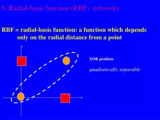
Learning from Examples • Learning from examples is natural in human beings • Central to the study and design of artificial neural systems. • Objective in understanding learning mechanisms • Develop software and hardware that can learn from examples and exploit information in impinging data. • Examples: • bit streams from radio telescopes around the globe • 100 TB on the Internet
Generalization • Supervised systems learn from a training set T = {Xk, Dk} Xkn, Dk • Basic idea: Use the system (network) in predictive mode ypredicted = f(Xunseen) • Another way of stating is that we require that the machine be able to successfully generalize. • Regression: ypredicted is a real random variable • Classification: ypredicted is either +1, -1
Approximation • Approximation results discussed in Chapter 6 give us a guarantee that with a sufficient number of hidden neuronsit should be possible to approximate a given function (as dictated by the input–output training pairs) to any arbitrary level of accuracy. • Usefulness of the network depends primarily on the accuracy of its predictions of the output for unseen test patterns.
Important Note • Reduction of the mean squared error on the training set to a low level does not guarantee good generalization! • Neural network might predict values based on unseen inputs rather inaccurately, even when the network has been trained to considerably low error tolerances. • Generalization should be measured using test patterns similar to the training patterns • patterns drawn from the same probability distribution as the training patterns.
Broad Objective • To model the generator function as closely as possible so that the network becomes capable of good generalization. • Not to fit the model to the training data so accurately that it fails to generalize on unseen data.
Networks with too many weights (free parameters) overfits training data too accurately and fail to generalize Example: 7 hidden node feedforward neural network 15 noisy patterns that describe the deterministic univariate function (dashed line). Error tolerance 0.0001. Network learns each data point extremely accurately Network function develops high curvature and fails to generalize Example of Overfitting
Occam’s Razor Principle • William Occam, c.1280–1349 • No more things should be presumed to exist than are absolutely necessary. • Generalization ability of a machine is closely related to • the capacity of the machine (functions it can represent) • the data set that is used for training.
Statistical Learning Theory • Proposed by Vapnik • Essential idea: Regularization • Given a finite set of training examples, the search for the best approximating function must be restricted to a small space of possible architectures. • When the space of representative functions and their capacity is large and the data set small, the models tend to over-fit and generalize poorly. • Given a finite training data set, achieve the correct balance between accuracy in training on that data set and the capacity of the machine to learn any data set without error.
Optimal Neural Network • Recall the sum of squares error function • Optimal neural network satisfies Residual error: average training data variance conditioned on the input The optimal network function we are in search of minimizes the error by trying to make the first integral zero
Training Dependence on Data • Network deviation from the desired average is measured by • Deviation depends on a particular instance of a training data set • Dependence is easily eliminated by averaging over the ensemble of data sets of size Q
Causes of Error: Bias and Variance • Bias: network function itself differs from the regression function E[d|X] • Variance: network function is sensitive to the selection of the data set • generates large error on some data sets and small errors on others.
Quantification of Bias & Variance • Consequently, = 0
Bias-Variance Dilemma • Separation of the ensemble average into the bias and variance terms: • Strike a balance between the ratio of training set size to network complexity such that both bias and variance are minimized. • Good generalization • Two important factors for valid generalization • the number of training patterns used in learning • the number of weights in the network
T is sampled stochastically Xk X n, dk D Xkdoes not map uniquely to an element, rather a distribution Unkown probability distribution p(X,d) defined on X D determines the probability of observing (Xk, dk) Stochastic Nature of T (T = {Xk, Dk} Xkn, Dk) dk Xk X P(X) D P(d|x)
Risk Functional • To successfully solve the regression or classification task, a neural network learns an approximatingfunctionf(X, W) • Define the expected risk as • The risk is a function of functions f drawn from a function space F Loss Function
Loss Functions • Square error function • Absolute error function • 0-1 Loss function
Optimal Function • The optimal function fo minimizes the expected risk R[f] • fo defined by optimal parameters; Wo is the ideal estimator • Remember: p(X,d) is unknown, and fo has to be estimated from finite samples • focannot be found in practice!
Empirical Risk Minimization (ERM) • To solve above problem, Vapnik suggested ERM principle • ERM principleis an induction principle that we can use to train the machine using the limited number of data samples at hand • ERM generates a stochastic approximation of R using T called the empirical risk Re
Empirical Risk Minimization (ERM) • The best minimizer of the empirical risk replaces the optimal function fo • ERM replaces R by Reand fo by • Question: • Is the minimizer close to fo?
Two Important Sequence Limits • To ensure minimizer close to fo,weneed to find the conditions for consistency of the ERM principle. • Essentially requires specifying the necessary and sufficient conditions for convergence of the following two limits of sequences in a probabilistic sense.
First Limit • Convergence of the values of expected risks of functions ,Q = 1,2,… that minimize the empirical risk over training sets of size Q, to the minimum of the true risk • Another way of saying that solutions found using ERM converge to the best possible solution.
Second Limit • Convergence of the values of empirical risk Q = 1,2,… over training sets of size Q, to the minimum of the true risk • This amounts to stating that the empirical risk converges to the value of the smallest risk. • Leads to the Key Theorem by Vapnik and Chervonenkis
Key Theorem • Let L(d,f(X,W)) be a set of functions with a bounded loss for probability measure p(X,d) : • Then for the ERM principle to be consistent, it is necessary and sufficient that the empirical risk Re[f] converge uniformly to the expected risk R[f] over the set L(d,f(X,W)) such that • This is called uniform one-sided convergence in probability
Points to Take Home • In the context of neural networks, each function is defined by the weights W of the network. • Uniform convergence Theorem and VC Theory ensure that W which is obtained by minimizing Re also minimizes R as the number Q of data points increases towards infinity.
Points to Take Home • Remember: we have a finite data set to train our machine. • When any machine is trained on a specific data set (which is finite) the function it generates is a biased approximant which may minimize the empirical risk or approximation error, but not necessarily the expected risk or the generalization error.
Indicator Functions and Labellings • Consider the set of indicator functions • F = {f(X,W)} mapping points inn into {0,1} or {-1,1}. • Labelling: An assignment of 0,1 to Q points in n • Q points can be labelled in 2Q ways
Labellings in 3-d (d) (c) (b) (a) (g) (h) (e) (f) Three points in R2 can be labelled in eight different ways. A linear oriented decision boundary can shatter all eight labellings.
Vapnik–Chervonenkis Dimension • If the set of indicator functions can correctly classify each of the possible 2Q labellings, we say the set of points is shattered by F. • The VC-dimensionh of a set of functionsFis the largest set of points that can be shattered by the set in question.
Labelling of four points in 2 that cannot be correctly separated by a linear oriented decision boundary A quadratic decision boundary can separate this labelling! VC-Dimension of Linear Decision Functions in 2 is 3
VC-Dimension of Linear Decision Functions in n • At most n+1 points can be shattered by oriented hyperplanes in n • VC-dimension is n+1 • Equal to the number of free parameters
Growth Function • Consider Q points in n • NXQ labellings can be shattered by F • NXQ 2Q • Growth function
Growth Function and VC Dimension G(Q) Nothing in between these is allowed The point of deviation is the VC-dimension h Q
Towards Complexity Control • In a machine trained on a given training set the appoximants generated are naturally biased towards those data points. • Necessary to ensure that the model chosen for representation of the underlying function has a complexity (or capacity) that matches the data set in question. • Solution: structural risk minimization • Consequence of VC-theory • The difference between the empirical and expected risk can be bounded in terms of the VC-dimension.
VC-Confidence, Confidence Level • For binary classification loss functions which take on values either 0,1, for some 01 the following bound holds with probability at least 1-: VC-confidence holds with confidence level 1- Empirical error
Structural Risk Minimization • Structural Risk Minimization (SRM): • Minimize the combination of the empirical risk and the complexity of the hypothesis space. • Space of functions F is very large, and so restrict the focus of learning to a smaller space called the hypothesisspace.
Structural Risk Minimization • SRM therefore defines a nested sequence of hypothesis spaces • F1 F2 … Fn … • VC-dimensions h1 h2 … hn … Increasing complexity
Nested Hypothesis Spaces form a Structure F1 F2 Fn F3 VC-dimensionsh1 h2 … hn …
Empirical and Expected Risk Minimizers • minimizes the empirical error over the Q points in space Fi • Is different from the true minimizer of the expected risk R in Fi
A Trade-off • Successive models have greater flexibility such that the empirical error can be pushed down further. • Increasing i increases the VC-dimension and thus the second term • Find Fn(Q), the minimizer of the r.h.s. • Goal: select an appropriate hypothesis space to match the training data complexity to the model capacity. • This gives the best generalization.
Approximation Error: Bias • Essentially two costs associated with the learning of the underlying function. • Approximation error, EA: • Introduced by restricting the space of possible functions to be less complex than the target space • Measured by the difference in the expected risks associated with the best function and the optimal function that measures R in the target space • Does not depend on the training data set; only on the approximation power of the function space
Estimation Error: Variance • Now introduce the finite training set with which we train the machine. • Estimation Error, EE: • Learning from finite data minimizes the empirical risk; not the expected risk. • The system thus searches a minimizer of the expirical risk; not the expected risk • This introduces a second level of error. • Generalization error = EA +EE
A Warning on Bound Accuracy • As the number of training points increase, the difference between the empirical and expected risk decreases. • As the confidence level increases ( becomes smaller), the VC confidence term becomes increasingly large. • With a finite set of training data, one cannot increase the confidence level indefinitely: • the accuracy provided by the bound decreases!
Origins • Support Vector Machines (SVMs) have a firm grounding in the VC theory of statistical learning • Essentially implements structural risk minimization • Originated in the work of Vapnik and co-workers at the AT&T Bell Laboratories • Initial work focussed on • optical character recognition • object recognition tasks • Later applications • regression and time series prediction tasks
Context • Consider two sets of data points that are to be classified into one of two classes C1, C2 • Linear indicator functions (TLN hyperplane classifiers) which is the bipolar signum function • Data set is linearly separable • T = {Xk, dk}, Xkn, dk {-1,1} • C1: positive samples C2: negative samples
Class 1 Class 1 Class 2 Class 2 SVM Design Objective • Find the hyperplane that maximizes the margin Distance to closest points on either side of hyperplane
Hypothesis Space • Our hypothesis space is the space of functions • Similar to Perceptron, but now we want to maximize the margins from the separating hyperplane to the nearest positive and negative data points. • Find the maximum margin hyperplanefor the given training set.
The perpendicular distance to the closest positive sample (d+) or negative sample (d-) is called the margin Definition of Margin Class 1 X+ d+ Class 2 d- X-