Graphing Linear Equations
150 likes | 391 Vues
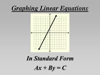
Graphing Linear Equations. In Slope-Intercept Form. We have already seen that linear equations have two variables and when we plot all the (x,y) pairs that make the equation true we get a line.

Graphing Linear Equations
E N D
Presentation Transcript
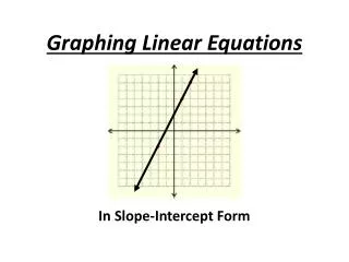
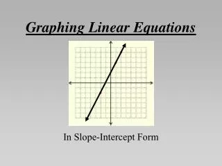
Graphing Linear Equations In Slope-Intercept Form
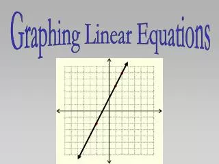
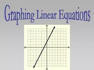
We have already seen that linear equations have two variables and when we plot all the (x,y) pairs that make the equation true we get a line. In this section, instead of making a table, evaluating y for each x, plotting the points and making a line, we will use The Slope-Intercept Form of the equation to graph the line.
These equations are all in Slope-Intercept Form: Notice that these equations are all solved for y.
Just by looking at an equation in this form, we can draw the line (no tables). • The constant is the y-intercept. • The coefficient is the slope. Constant = 1, y-intercept = 1. Coefficient = 2, slope = 2. Constant = -4, y-intercept = -4. Coefficient = -1, slope = -1. Constant = -2, y-intercept = -2. Coefficient = 3/2, slope = 3/2.
The formula for Slope-Intercept Form is: • ‘b’ is the y-intercept. • ‘m’ is the slope. On the next three slides we will graph the three equations: using their y-intercepts and slopes.
right 1 up 2 right 1 up 2 1) Plot the y-intercept as a point on the y-axis. The constant, b = 1, so the y-intercept = 1. 2) Plot more points by counting the slope up the numerator (down if negative) and right the denominator. The coefficient, m = 2, so the slope = 2/1.
down 1 down 1 right 1 right 1 1) Plot the y-intercept as a point on the y-axis. The constant, b = -4, so the y-intercept = -4. 2) Plot more points by counting the slope up the numerator (down if negative) and right the denominator. The coefficient, m = -1, so the slope = -1/1.
right 2 up 3 right 2 up 3 1) Plot the y-intercept as a point on the y-axis. The constant, b = -2, so the y-intercept = -2. 2) Plot more points by counting the slope up the numerator (down if negative) and right the denominator. The coefficient, m = 3/2, so the slope = 3/2.
Sometimes we must solve the equation for y before we can graph it. The constant, b = 3 is the y-intercept. The coefficient, m = -2 is the slope.
down 2 down 2 right 1 right 1 1) Plot the y-intercept as a point on the y-axis. The constant, b = 3, so the y-intercept = 3. 2) Plot more points by counting the slope up the numerator (down if negative) and right the denominator. The coefficient, m = -2, so the slope = -2/1.
HW • pg. 297 #2,4,6,8,10 • pg. 298 #12 to 26 even