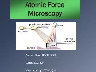
Atomic Force Microscopy

1. Atomic Force Microscopy • Lecture 7 Outline 1. Introduction to Atomic Forces2. AFM Modes of operation 3. Case study 11: Information from AFM

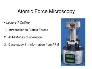
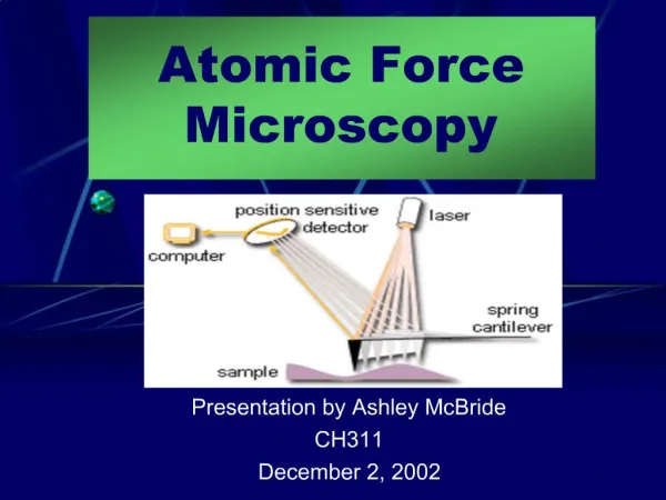
2. Atomic Force Microscopy • Both STM and atomic force microscopy (AFM) are part of the scanning probe microscope family. • STM uses the electronic properties between the tip and the sample. • AFM uses Forces between the sample and a tip on the end of a cantilever. These forces change as the tip gets closer to the sample. • So what are these forces???

3. Atomic Forces Force versus distance Force Repulsive force Tip-to-sample separation d 1/d8 1/d7 attractive force Fig. 7.1 Force - distance curve

4. Let us analyze what is going on in this curve… • 1. As the atoms are gradually brought together, they first weakly attract each other (1/d8). • 2. Attraction increases (1/d7) until the atoms are so close together that their electron clouds begin to repel each other electrostatically.

5. 3 The force goes to zero when the distance between the atoms reaches a couple of angstroms, • = about the length of a chemical bond. • When the total van der Waals force becomes positive (repulsive), the atoms are in contact.

6. 4. The slope of the Force curve is very steep in the repulsive or contact regime.  As a result, the repulsive force balances almost any force that attempts to push the atoms closer together.  In AFM this means that when the cantilever pushes the tip against the sample, the cantilever bends rather than forcing the tip atoms closer to the sample atoms.

7. Fig. 7.2 AFM cantilever

8. In practice • An atomically sharp tip is scanned over a surface with feedback mechanisms that enable the piezoelectric scanners to maintain the tip at either • (i) a constant force (to obtain height information), • (ii) or height (to obtain force information) above the sample surface. • Tips are typically made from Si3N4 or Si, and extended down from the end of a cantilever.

9. Modes of operation. There are 3 modes of AFM operation • Contact mode • Non-contact mode • Tapping mode Contact mode Non-contact mode Tapping mode Fig. 7.3 Modes

10. Contact mode: • The tip is moved over the surface by the scanning system. • A value of the cantilever deflection, for example, is selected and then the feedback system adjusts the height of the cantilever base to keep this deflection constant as the tip moves over the surface. • Non-contact mode: • The cantilever oscillates close to the sample surface, but without making contact with the surface. • The capillary force makes this particularly difficult to control in ambient conditions. Very stiff cantilevers are needed.

11. Tapping mode • The cantilever oscillates and the tip makes repulsive contact with the surface of the sample at the lowest point of the oscillation. • Tapping mode is useful for imaging soft samples such as biology or polymers. • Oscillation  resonance condition important

12. The cantilever is usually driven close to a resonance of the system. • The phase of the cantilever oscillation can give information about the sample properties, such as stiffness and mechanical information or adhesion. • Resonant frequency of the cantilever depends on its mass and spring constant; stiffer cantilevers have higher resonant frequencies.

13. Resonance frequency Phase Amplitude Frequency Question: Where would you want to operate system at??? At resonance? Fig. 7.4

14. Cantilever spring constant k Cantilever deflection s s F = k s Force F Fig. 7.5

15. Used to measure long range attractive or repulsive forces between the probe tip and the sample surface. • Force curves( force-versus-distance curve) typically show the deflection of the free end of the AFM cantilever as the fixed end of the cantilever is brought vertically towards and then away from the sample surface. • The deflection of the free end of the cantilever is measured and plotted at many points as the z-axis scanner extends the cantilever towards the surface and then retracts it again..

16. Force measurements. The AFM can record the amount of force felt by the cantilever as the probe tip is brought close to - and even indented into - a sample surface and then pulled away Fig. 7.6 Force distance

17. Consider a cantilever in air approaching a hard, incompressible surface such as glass or mica. AB: As the cantilever approaches the surface, initially the forces are too small to give a measurable deflection of the cantilever, and the cantilever remains in its undisturbed position. BC: At some point, the attractive forces (usually Van der Waals, and capillary forces) overcome the cantilever spring constant and the tip jumps into contact with the surface.

18. CD: Once the tip is in contact with the sample, it remains on the surface as the separation between the base and the sample decreases further, causing a deflection of the tip and an increase in the repulsive contact force. DF, FG: As the cantilever is retracted from the surface, often the tip remains in contact with the surface due to some adhesion and the cantilever is deflected downwards. GH: At some point the force from the cantilever will be enough to overcome the adhesion, and the tip will break free.

19. Applications Molecular interactions

20. Phase Amplitude Tapping mode Frequency Modern AFM imaging – phase imaging. In tapping mode, we vibrate the cantilever and we have resonance frequency. Nornally we ignore any thing to do with the phase, however there is now a lot of research in using phase imaging to go beyond simple topographical mapping to detect variations in composition, adhesion, friction, viscoelasticity. Fig. 7.7 Phase imaging

21. Some examples of phase imaging. Fig. 7.9 Bond pad on an integrated circuit imaged by TappingMode (left) and phase (right). Pad contaminated with polyimide produce light contrast with phase shifts of over 120 deg. 1.5 µm scan Fig. 7.10 Tapping Mode (L) and phase images (R) of a composite polymer embedded in a uniform matrix

22. AFM vs STM • Resolution of STM is better than AFM because of the exponential dependence of the tunneling current on distance. • STM is generally applicable only to conducting samples while AFM is applied to both conductors and insulators. • AFM offers the advantage that the writing voltage and tip-to-substrate spacing can be controlled independently, whereas with STM the two parameters are integrally linked.

23. Other types of SPM MFM – Magnetic Force Microscopy Fig. 7.11 The dots are made of permalloy and are 400 nm apart. The MFM image gives the field distribution for a non polarized sample, and a few different configuration are observed. EFM – Electric Force Microscopy Field of view 10µm x 10µm Fig. 7.12 Different types of material are deposited on Si wafers during processing.

24. Scanning Capacitance Microscopy SCM Fig. 7.13 shows two sets of AFM measurements (topography and SCM) for a correctly aligned mask(left) and for a misaligned mask (right). The large pictures are a combination of both the topography (grey) and the SCM image (orange). From these images the amount and direction of the misalignment can be observed. Field of view 30µm x 30µm

25. Using AFMs as tools I: Dip-pen Nanolithography • “In the year 2000, …, they will wonder why it was not until the year 1960 that anybody began seriously to move in this direction (miniaturization)." Richard Feynman

26. Dip-pen Nanolithography Fig. 7.14 DPN

27. http://www.chem.northwestern.edu/~mkngrp/dpn.htm

28. Using AFMs as tools: II Nanomanipulation "NanoMan and Best Friend" DNA strand 400 x 480 nm scans showing carbon nanotube manipulation

29. Summary • AFM uses force to probe the surface topology and properties of materials. • Tapping modes vs Contact mode • Phase imaging is a modern way to prove extra information. • Dip- pen nanolithography is a way to perform serial writing.